
 By Islam Baraka
The governed definitions this build depends on. Read them first if a term is unfamiliar.
- PrimarySimple Moving AverageSimple Moving Average is the arithmetic mean of observations in a declared moving window.
- PrerequisiteRolling WindowRolling Window is an ordered observation subset whose endpoints move as new data becomes eligible.
- ImportantCausal Knowledge CutoffThe time boundary that prevents information unavailable at that moment from influencing a calculation.
- ImportantFull-Window ReadinessFull-Window Readiness means an algorithm emits a valid value only after receiving its complete declared observation window.
- ImportantMoving AverageMoving Average is a smoothing statistic recomputed or recursively updated as the observation position advances.
- ImportantMoving-Average LookbackMoving-Average Lookback is the declared window length and calendar basis used by a moving-average calculation.
- ImportantNo-Imputation Missing-Session PolicyA policy that blocks or pauses calculation instead of converting a missing required session into a zero observation.
- ImportantReady PointThe first eligible observation at which every state required for an indicator output has been initialized.
- ImportantSuffix RecalculationRecomputing a corrected observation and every later output whose recursive state may depend on it.
- ImportantWarm-Up PeriodThe initial span in which an indicator is accumulating enough eligible history to satisfy its declared initialization policy.
Six observations arrive:
The latest value is 18. Is the recent level 18? Not necessarily. One observation can be noisy, so we ask a more stable question:
What is the average of the latest three accepted observations?
At the sixth observation, those values are 15, 14, and 18:
That is a three-observation Simple Moving Average. The arithmetic is elementary. The contract around the arithmetic is where robust financial software begins.
The learning promise
By the end, you will be able to:
- identify exactly which values enter a finance-style SMA;
- calculate it directly or with a constant-time rolling update;
- explain why early nulls, missing timestamps, and adjusted prices matter;
- distinguish causal SMA from centered, partial-window, cumulative, and time-based variants;
- implement matching Python and TypeScript versions;
- understand why SMA is the right prerequisite for EMA.
One formula, several hidden choices
For a window of observations:
Here:
- is the current accepted observation;
- is a positive integer window length;
- counts accepted observations, not necessarily calendar days;
- the result is attached to the newest point in the window.
This is a trailing or right-aligned average. It uses the current observation and earlier observations. It is causal because it never uses a value after .
Every window member has the same weight:
and the weights sum to one:
That gives the SMA two useful properties.
First, shifting every value by the same constant shifts the SMA by that constant. Second, the result must lie between the smallest and largest values in the active window:
If a calculated SMA lies outside that range, something is wrong with the data, window membership, or implementation.
“Moving” means replacement
Start with the first complete three-value window:
so:
One observation later, the window is no longer . Value 10 leaves, values 13 and 12 stay, and value 15 enters:
The direct calculation is correct, but repeatedly summing all values costs work per output. A rolling sum expresses the window movement directly:
For observation 4:
and:
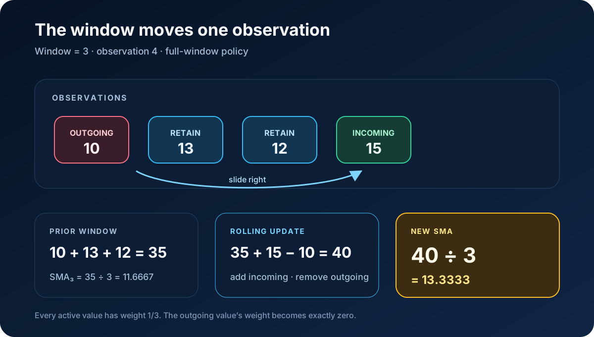
The incoming/outgoing bookkeeping is the direct mean reorganized, not a different estimator. Open the diagram at full size.
The rolling recurrence is not an approximation to the direct formula. In exact arithmetic, it is the same formula reorganized. It turns the per-observation calculation into work.
The complete example
Use:
The canonical full-window calculation is:
| Observation | Active window | Update | SMA |
|---|---|---|---|
| 1 | 10 | Not enough values | null |
| 2 | 10, 13 | Not enough values | null |
| 3 | 10, 13, 12 | 11.6667 | |
| 4 | 13, 12, 15 | 13.3333 | |
| 5 | 12, 15, 14 | 13.6667 | |
| 6 | 15, 14, 18 | 15.6667 |
The full-precision output is:
[null, null, 11.666666666666666, 13.333333333333334,
 13.666666666666666, 15.666666666666666]
The raw series moves down at observation 3 and observation 5. The three-point SMA changes more gradually because every result combines three observations.
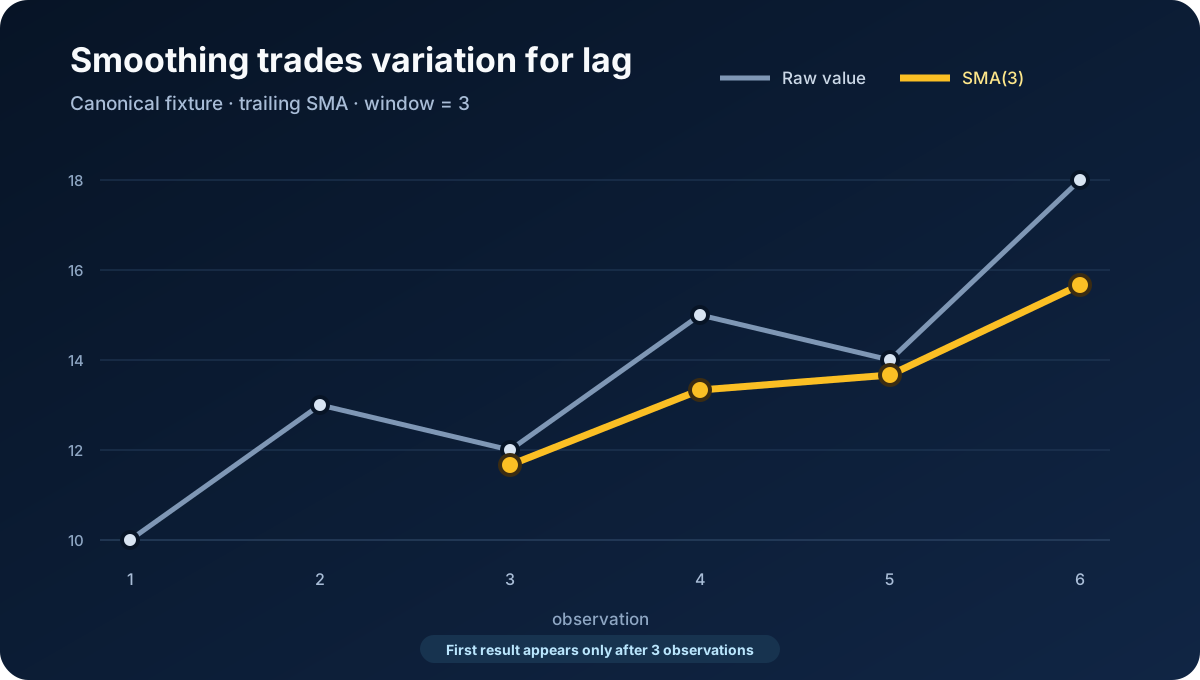
The three-observation line starts only after warm-up and changes more gradually than the synthetic raw values. It demonstrates smoothing and lag, not predictive success. Open the chart at full size.
This smoothness has a cost: lag. At observation 6, the raw value has reached 18 while the SMA is 15.6667. A longer window usually reduces short-run variation more strongly, but it also waits longer for readiness and responds more slowly to a new level.
Warm-up is part of the answer
At observation 1, the system has one value—not three. At observation 2, it has two. The canonical result is null for both.
Why not calculate and ? You can, but that is a partial-window mean:
Its denominator changes during warm-up. The first result averages one value, the next averages two, and later values average three. Those early outputs do not have the same statistical meaning as the declared three-observation SMA.
This package therefore sets:
minimum_periods = window
and emits null until readiness. pandas exposes this choice explicitly through rolling-window parameters, and its fixed-window examples show nulls before the first complete mean. A production API should do the same rather than hiding a default.
The playground includes partial-window behavior for comparison, but labels it as a variant.
Try window lengths 1 through 5. Notice three linked effects:
- a larger window takes longer to produce its first canonical result;
- it combines more observations;
- it generally creates a smoother, slower-moving line.
Trailing and centered averages are not interchangeable
A centered three-point average at observation uses:
The future value is part of the result labeled at . Centering is useful for retrospective trend-cycle estimation, but it is not available in real time at the centered timestamp.
A trading study that calculates a centered average and acts as though it was known at contains look-ahead bias.
The canonical finance SMA is trailing:
It uses only information available by the close of observation , assuming the source point itself is final and the decision timing allows its use.
Observation windows are not time windows
Suppose daily values exist on Friday, Monday, and Tuesday. A three-observation SMA contains those three accepted sessions. The weekend does not add two zero observations.
This is a fixed-count contract:
window = 3 accepted observations
A time-based rolling rule such as “all observations in the previous 72 hours” is different. Its count can change across weekends, holidays, outages, and irregular event streams.
Neither choice is universally right. The error is describing one and implementing the other.
For market data, record:
- calendar identity;
- frequency;
- timezone and timestamp meaning;
- whether the timestamp represents open, close, settlement, or publication;
- how missing sessions and halted instruments are represented.
A bounded historical example: official SOFR observations
The Federal Reserve Bank of New York publishes the Secured Overnight Financing Rate (SOFR) on business days. Its Markets API returned the following effective-date observations for 2–8 January 2024. The SOFR values are provider observations; the SMA values are arithmetic derived for this article.
| Effective date | New York Fed SOFR (%) | Author-derived SMA(3) (%) |
|---|---|---|
| 2024-01-02 | 5.40 | null |
| 2024-01-03 | 5.39 | null |
| 2024-01-04 | 5.32 | 5.3700 |
| 2024-01-05 | 5.31 | 5.3400 |
| 2024-01-08 | 5.31 | 5.3133 |
The 8 January result uses the three accepted observations dated 4, 5, and 8 January:
The weekend does not add two zeros or two carried-forward copies. This is the concrete difference between a three-observation window and a three-calendar-day rule.
The New York Fed's reference-rate publication policy says an initially published reference rate can be revised later the same day under defined conditions. A production SMA should therefore retain observation and revision provenance. Nothing in this five-row example establishes a forecast, signal, causal event, or trading result. The reproducibility record—endpoint parameters, retrieval time, response hash, exact provider values, and derived arithmetic—is stored in the package dataset.
Missing data is not zero
Numeric zero can be a valid observation. Net Advances can be zero. A rate can be zero. A price may not normally be zero, but replacing a missing price with zero would still be a data corruption, not an SMA rule.
This package rejects:
- null;
- NaN;
- positive or negative infinity;
- booleans;
- numeric strings.
An absent timestamp creates no update. The canonical observation-space SMA neither inserts a zero nor carries the last value forward.
If imputation is required, treat it as an upstream transformation with its own provenance. The output then describes an SMA of the imputed series, not an SMA of the original observations.
Price basis can break a window
Imagine four unadjusted closes followed by a two-for-one stock split. The mechanical price drop can dominate a rolling average even though shareholder value did not halve. Mixing unadjusted history with an adjusted current value is worse: the window no longer has a coherent unit basis.
Choose and preserve a value_basis, such as:
- raw close;
- split-adjusted close;
- total-return adjusted close;
- settlement price;
- a named vendor field and adjustment version.
If the source revises its history, every SMA whose window contains a revised observation can change. For window , one revised point can affect up to right-aligned outputs.
Provisional values need window-local provenance
Suppose today’s input is provisional. Today’s SMA is provisional because that value belongs to its active window. Tomorrow’s and later SMAs remain provisional until the unresolved value exits or becomes final.
For a finite-window SMA, provisional influence has a clear boundary. This differs from a recursive EMA, where a revised observation can influence all later states unless the series is recomputed or state is corrected.
A useful output row therefore carries:
- whether the current source value is provisional;
- whether any observation in the active window is provisional;
- the active window’s start and end;
- source revision or snapshot identifiers.
Reference implementation
The Python core:
def calculate_sma(values, window):
    if not isinstance(window, int) or isinstance(window, bool) or window < 1:
        raise SMAValidationError("window must be a positive integer.")

    numbers = validate_finite_values(values)
    result = []
    rolling_sum = 0.0

    for index, value in enumerate(numbers):
        rolling_sum += value
        if index >= window:
            rolling_sum -= numbers[index - window]
        result.append(None if index + 1 < window else rolling_sum / window)

    return result
The TypeScript version uses the same branch structure:
export function calculateSma(
  values: readonly number[],
  window: number,
): Array<number | null> {
  validateWindowAndValues(values, window);
  const output: Array<number | null> = [];
  let rollingSum = 0;

  values.forEach((value, index) => {
    rollingSum += value;
    if (index >= window) rollingSum -= values[index - window];
    output.push(index + 1 < window ? null : rollingSum / window);
  });
  return output;
}
The package implementation expands the validation helpers and uses one JSON fixture set for both languages. A second boundary function, calculate_sma_series in Python and calculateSmaSeries in TypeScript, validates timestamp order, source identity, unit, calendar, frequency, value basis, and finality before producing auditable rows. The short array function above remains the intentionally narrow numeric core.
Numerical behavior
The formula should keep full floating-point precision. Rounding every SMA for display is fine; rounding the rolling sum before the next update is not.
Binary floating-point cannot represent every decimal fraction exactly, and repeated add/subtract updates can accumulate small error in very long streams. Three practical controls are:
- define an absolute and relative tolerance in tests;
- periodically rebuild the sum from the retained window when the error budget requires it;
- use compensated summation for demanding magnitude ranges.
Do not introduce a different numerical policy in only one language. Cross-language parity is part of reproducibility.
Tests that catch semantic errors
Arithmetic tests are necessary, but contract tests catch more dangerous failures.
Canonical fixture
Verify every output, including the first two nulls.
Window one
If that fails, indexing or readiness is wrong.
Window longer than history
Every canonical output must be null.
Translation invariance
For constant :
This catches some membership and denominator mistakes.
Range invariant
Every ready result must remain between the active window’s minimum and maximum.
Invalid data
Reject invalid windows, null-like values, NaN, infinity, booleans, and ambiguous strings.
Direct-versus-rolling check
For generated finite sequences, compare each rolling output with an independently summed window within the declared tolerance.
Provenance and historical arithmetic
Reject duplicate or decreasing timestamps and any mid-run change in series identity, unit, calendar, frequency, or value basis. Verify that provisional state persists exactly while the provisional source row remains inside a ready window. Recalculate the five-row New York Fed illustration from the stored provider observations rather than treating its displayed rounded values as test inputs.
Common mistakes
Calling a cumulative mean an SMA
A cumulative average uses all history:
Its memory grows. An SMA’s memory remains .
Treating 20 as calendar days
Most finance chart conventions mean 20 accepted observations. A time-duration window needs a different API and tests.
Silently emitting partial windows
Early numbers look plausible but use changing denominators.
Centering a backtest feature
The line looks visually balanced because it uses future data.
Rounding state
Presentation precision leaks into calculation and creates platform disagreement.
Mixing adjustment bases
The window averages quantities that are not economically comparable.
Confusing smoothing MA with MA()
In time-series modeling, a moving-average model combines current and past random shocks. It is not this rolling mean of observed prices or indicators.
What SMA can and cannot tell you
SMA can answer:
- What is the equal-weight mean of the latest accepted observations?
- Is the current observation above or below that recent mean?
- How has a smoothed historical level changed?
SMA alone cannot answer:
- Will the next price rise?
- Is a chosen window optimal?
- Will a crossover remain profitable after costs?
- Is a structural break temporary or permanent?
- Is the source history free of survivorship or revision bias?
Those require separate models, evaluation, and controls.
The bridge to EMA
SMA has a hard window edge. A value has weight while it remains inside, then its weight becomes exactly zero.
EMA behaves differently. It updates recursively:
Older influence decays geometrically rather than disappearing at a single window boundary. In the canonical EMA topic, the first state is seeded with the SMA of the first observations.
That makes SMA the right first topic. Once you understand:
- what a window contains;
- when a full result exists;
- why input order and basis matter;
- how a seed is calculated;
you can focus on the genuinely new EMA ideas: alpha, persistence, recursive state, and infinite theoretical memory.
Final checklist
Before accepting an SMA implementation, ask:
- Is the window fixed-count or elapsed-time?
- Is it trailing or centered?
- Is the label attached to the newest point?
- Must a full window exist?
- What happens to missing values and missing timestamps?
- Are values finite and consistently adjusted?
- Is zero treated as data?
- Is precision retained internally?
- Can revisions be traced and recomputed?
- Do Python and TypeScript match the same fixture?
If those answers are explicit, the Simple Moving Average is not just a formula. It is a reproducible financial data contract.
References
Definitions and convention evidence are documented in REFERENCES.md, including NIST sources for moving-average smoothing and centering, pandas rolling-window semantics, and official New York Fed sources for the bounded SOFR illustration and revision timing.
Rendered from the canonical Mermaid sources linked by this article.
SMA calculation flow
The canonical branch emits null until a complete fixed-count window exists. The same branch then remains causal by removing only the oldest accepted observation.
The result is right-aligned at the current observation. No future value enters the branch.
ReferencesPrimary sources and evidence notesExpand the source trail, evidence role, and limitations behind the engineering choices.
Expand the source trail, evidence role, and limitations behind the engineering choices.
NIST-01 — Single Moving Average
- Organization or authors: NIST/SEMATECH
- Source type: Official engineering-statistics handbook
- Publication or effective date: Undated living handbook
- Version: Web edition
- URL or DOI: https://www.itl.nist.gov/div898/handbook/pmc/section4/pmc421.htm
- Accessed: 2026-07-23
- Jurisdiction: Not jurisdiction-specific
- Supports: Successive fixed-size subsets, the trailing moving-average formula, advancing one period, and dropping the oldest value
- Limitations: General time-series treatment; it does not define finance-specific timestamp, adjustment, or finality policies
NIST-02 — Averaging Methods
- Organization or authors: NIST/SEMATECH
- Source type: Official engineering-statistics handbook
- Publication or effective date: Undated living handbook
- Version: Web edition
- URL or DOI: https://www.itl.nist.gov/div898/handbook/pmc/section4/pmc42.htm
- Accessed: 2026-07-23
- Jurisdiction: Not jurisdiction-specific
- Supports: Arithmetic-mean calculation, equal weights, and weights summing to one
- Limitations: Discusses smoothing broadly and does not prescribe the package's full-window API contract
NIST-03 — Centered Moving Average
- Organization or authors: NIST/SEMATECH
- Source type: Official engineering-statistics handbook
- Publication or effective date: Undated living handbook
- Version: Web edition
- URL or DOI: https://www.itl.nist.gov/div898/handbook/pmc/section4/pmc422.htm
- Accessed: 2026-07-23
- Jurisdiction: Not jurisdiction-specific
- Supports: Centered placement and use of observations on both sides of the labeled point
- Limitations: Centered smoothing is a comparison variant, not the canonical causal algorithm in this package
NIST-04 — Common Approaches to Univariate Time Series
- Organization or authors: NIST/SEMATECH
- Source type: Official engineering-statistics handbook
- Publication or effective date: Undated living handbook
- Version: Web edition
- URL or DOI: https://www.itl.nist.gov/div898/handbook/pmc/section4/pmc444.htm
- Accessed: 2026-07-23
- Jurisdiction: Not jurisdiction-specific
- Supports: Distinguishing the statistical MA(q) model over random shocks from rolling smoothing of observed values
- Limitations: Does not define technical-indicator conventions
PANDAS-01 — DataFrame.rolling
- Organization or authors: pandas project
- Source type: Official library documentation
- Publication or effective date: Current documentation
- Version: Stable documentation accessed 2026-07-23
- URL or DOI: https://pandas.pydata.org/pandas-docs/stable/reference/api/pandas.DataFrame.rolling.html
- Accessed: 2026-07-23
- Jurisdiction: Not jurisdiction-specific
- Supports: Fixed-count versus time-based windows,
min_periods, centering, endpoint closure, and label semantics - Limitations: Library options are implementation variants, not universal finance defaults
PANDAS-02 — Rolling.mean
- Organization or authors: pandas project
- Source type: Official library documentation
- Publication or effective date: Current documentation
- Version: Stable documentation accessed 2026-07-23
- URL or DOI: https://pandas.pydata.org/docs/reference/api/pandas.core.window.rolling.Rolling.mean.html
- Accessed: 2026-07-23
- Jurisdiction: Not jurisdiction-specific
- Supports: Independently reproducible rolling-mean behavior and numerical output
- Limitations: Does not establish data provenance, market timing, or predictive value
NYFED-01 — Secured Overnight Financing Rate Data
- Organization or authors: Federal Reserve Bank of New York
- Source type: Official reference-rate data page
- Publication or effective date: Daily business-day publication
- Version: Web page accessed 2026-07-23
- URL or DOI: https://www.newyorkfed.org/markets/reference-rates/sofr
- Accessed: 2026-07-23
- Jurisdiction: United States
- Supports: SOFR definition, official publisher, business-day publication, and source role for the bounded historical observations
- Limitations: The source does not endorse the article's author-derived SMA or any forecasting interpretation
NYFED-02 — Markets Data APIs
- Organization or authors: Federal Reserve Bank of New York
- Source type: Official API documentation
- Publication or effective date: Current API documentation
- Version: Accessed 2026-07-23
- URL or DOI: https://markets.newyorkfed.org/static/docs/markets-api.html
- Accessed: 2026-07-23
- Jurisdiction: United States
- Supports: Reproducible retrieval of the 2–8 January 2024 SOFR observation window
- Limitations: Provider responses may be revised; the package records retrieval time and response hash
NYFED-03 — Additional Information about Reference Rates
- Organization or authors: Federal Reserve Bank of New York
- Source type: Official methodology and publication-policy page
- Publication or effective date: Current policy page
- Version: Accessed 2026-07-23
- URL or DOI: https://www.newyorkfed.org/markets/reference-rates/additional-information-about-reference-rates
- Accessed: 2026-07-23
- Jurisdiction: United States
- Supports: Business-day publication and the stated same-day revision process for Treasury repo reference rates
- Limitations: Policies can change; production systems should retain source snapshots and review current terms
Source-to-claim map
| Claim | Primary support |
|---|---|
| A trailing SMA advances one observation and drops the oldest value. | NIST-01 |
| Every member of an arithmetic mean has equal weight and the weights sum to one. | NIST-02 |
| A centered moving average uses values on both sides of its label and is retrospective. | NIST-03 |
| A statistical MA(q) model is not the rolling average taught here. | NIST-04 |
| Fixed-count, elapsed-time, centering, and minimum-period rules are distinct software contracts. | PANDAS-01 |
| The five SOFR values are official provider observations returned for the declared window. | NYFED-01, NYFED-02 |
| New York Fed reference-rate publication can include a defined same-day revision process. | NYFED-03 |
Reproducibility boundary
- Synthetic fixture:
[10, 13, 12, 15, 14, 18], window3, expected[null, null, 35/3, 40/3, 41/3, 47/3]. - Historical fixture: New York Fed SOFR effective dates 2024-01-02 through 2024-01-08, endpoint and non-secret parameters recorded in
datasets/sofr-2024-01-02-to-2024-01-08.json. - Provider observations and author-derived SMA values are stored in separate fields.
- Neither fixture establishes predictive ability, profitability, optimal parameters, or causation.
Full dependency-light reference implementations in both supported languages.
/** Canonical trailing simple moving average for D07-F01-A01. */

export class SMAValidationError extends Error {
  constructor(message: string) {
    super(message);
    this.name = "SMAValidationError";
  }
}

export interface SMAInputRecord {
  timestamp: string;
  value: number;
  series_id: string;
  unit: string;
  calendar: string;
  frequency: string;
  value_basis: string;
  is_final: boolean;
  source_snapshot_id: string;
  source_revision_id: string;
}

export interface SMAOutputRow {
  timestamp: string;
  value: number;
  sma: number | null;
  status: "warming" | "ready";
  observation_count: number;
  window: number;
  window_start: string | null;
  window_end: string | null;
  window_sum: number | null;
  source_is_provisional: boolean;
  source_snapshot_id: string;
  source_revision_id: string;
  sma_is_provisional: boolean | null;
  metric: "simple_moving_average";
}

export function calculateSma(
  values: readonly number[],
  window: number,
): Array<number | null> {
  if (!Number.isSafeInteger(window) || window < 1) {
    throw new SMAValidationError("window must be a positive integer.");
  }
  if (!Array.isArray(values)) {
    throw new SMAValidationError("values must be an array.");
  }

  const numbers = values.map((value, index) => {
    if (typeof value !== "number" || !Number.isFinite(value)) {
      throw new SMAValidationError(`values[${index}] must be a finite number.`);
    }
    return value;
  });

  const output: Array<number | null> = [];
  let rollingSum = 0;

  numbers.forEach((value, index) => {
    rollingSum += value;
    if (index >= window) rollingSum -= numbers[index - window];
    output.push(index + 1 < window ? null : rollingSum / window);
  });
  return output;
}

const identityFields = [
  "series_id",
  "unit",
  "calendar",
  "frequency",
  "value_basis",
  "source_snapshot_id",
] as const;

function validateTimestamp(value: unknown, index: number): number {
  if (typeof value !== "string" || value.trim() === "") {
    throw new SMAValidationError(`records[${index}].timestamp must be an RFC 3339 string.`);
  }
  if (!/(?:Z|[+-]\d{2}:\d{2})$/.test(value)) {
    throw new SMAValidationError(`records[${index}].timestamp must include an offset.`);
  }
  const parsed = Date.parse(value);
  if (!Number.isFinite(parsed)) {
    throw new SMAValidationError(`records[${index}].timestamp must be an RFC 3339 string.`);
  }
  return parsed;
}

export function calculateSmaSeries(
  records: readonly SMAInputRecord[],
  window: number,
): {
  metric: "simple_moving_average";
  window: number;
  series: Pick<
    SMAInputRecord,
    "series_id" | "unit" | "calendar" | "frequency" | "value_basis" | "source_snapshot_id"
  > | null;
  rows: SMAOutputRow[];
} {
  if (!Number.isSafeInteger(window) || window < 1) {
    throw new SMAValidationError("window must be a positive integer.");
  }
  if (!Array.isArray(records)) {
    throw new SMAValidationError("records must be an array.");
  }
  if (records.length === 0) {
    return { metric: "simple_moving_average", window, series: null, rows: [] };
  }

  let firstIdentity: Record<(typeof identityFields)[number], string> | null = null;
  let previousTimestamp: number | null = null;
  const validated = records.map((record, index) => {
    if (record === null || typeof record !== "object" || Array.isArray(record)) {
      throw new SMAValidationError(`records[${index}] must be an object.`);
    }
    const parsedTimestamp = validateTimestamp(record.timestamp, index);
    if (previousTimestamp !== null && parsedTimestamp <= previousTimestamp) {
      throw new SMAValidationError("timestamps must be unique and strictly increasing.");
    }
    previousTimestamp = parsedTimestamp;

    const identity = {} as Record<(typeof identityFields)[number], string>;
    for (const field of identityFields) {
      const value = record[field];
      if (typeof value !== "string" || value.trim() === "") {
        throw new SMAValidationError(`records[${index}].${field} must be non-empty.`);
      }
      identity[field] = value;
    }
    if (firstIdentity === null) firstIdentity = identity;
    else {
      for (const field of identityFields) {
        if (identity[field] !== firstIdentity[field]) {
          throw new SMAValidationError(`${field} must remain stable within one run.`);
        }
      }
    }

    if (typeof record.is_final !== "boolean") {
      throw new SMAValidationError(`records[${index}].is_final must be boolean.`);
    }
    if (typeof record.source_revision_id !== "string" || record.source_revision_id.trim() === "") {
      throw new SMAValidationError(`records[${index}].source_revision_id must be non-empty.`);
    }
    if (typeof record.value !== "number" || !Number.isFinite(record.value)) {
      throw new SMAValidationError(`records[${index}].value must be a finite number.`);
    }
    return { ...record };
  });

  const values: number[] = [];
  const rows: SMAOutputRow[] = [];
  let rollingSum = 0;

  validated.forEach((record, index) => {
    values.push(record.value);
    rollingSum += record.value;
    if (index >= window) rollingSum -= values[index - window];
    const ready = index + 1 >= window;
    const startIndex = Math.max(0, index - window + 1);
    const activeRecords = validated.slice(startIndex, index + 1);
    rows.push({
      timestamp: record.timestamp,
      value: record.value,
      sma: ready ? rollingSum / window : null,
      status: ready ? "ready" : "warming",
      observation_count: index + 1,
      window,
      window_start: ready ? activeRecords[0].timestamp : null,
      window_end: ready ? record.timestamp : null,
      window_sum: ready ? rollingSum : null,
      source_is_provisional: !record.is_final,
      source_snapshot_id: record.source_snapshot_id,
      source_revision_id: record.source_revision_id,
      sma_is_provisional: ready
        ? activeRecords.some((item) => !item.is_final)
        : null,
      metric: "simple_moving_average",
    });
  });

  return {
    metric: "simple_moving_average",
    window,
    series: firstIdentity,
    rows,
  };
}
The embedded lab now expands to its full document height, keeping the article as the only scroll surface.