D14-F03-A03 / Released engineering topic

Robust Mean-Variance: Make the Uncertainty Set Visible Before Trusting the Weights

A production-minded guide to Robust Mean-Variance.

By Islam Baraka 7 min read Reviewed Sep 15, 2026 Updated Sep 15, 2026 Python + TypeScript

Robust Mean-Variance: Make the Uncertainty Set Visible Before Trusting the Weights

D14 / D14-F03

“Robust” is one of the easiest words to add to an optimizer and one of the hardest claims to audit. A covariance matrix was shrunk. A penalty was added. The weights became less concentrated. None of those observations tells me what uncertainty the optimizer was designed to survive.

In this tutorial, robust has a precise meaning. The estimated mean is allowed to move inside a declared ellipsoid. For every candidate portfolio, an adversary chooses the mean inside that set that hurts the portfolio most. The optimizer balances that worst-case mean return against variance.

You will derive the penalty directly from the set, reproduce the optimum, see the adversarial mean direction, and verify that radius zero gives ordinary mean-variance. You will also see the method's honest limit: it protects against the uncertainty we modeled, not every future market state.

Start with the uncertainty set

Let mu_hat be the estimated mean. Define

U={mu_hat+Q u : ||u||_2<=kappa}.

The matrix Q gives the ellipsoid its directions and scale. The radius kappa sets how far the adversary may move in the dimensionless u coordinates. If Q says asset A's mean is twice as uncertain as asset B's, the geometry should show that. If a system cannot display Q and kappa, its “robust” label is not reproducible.

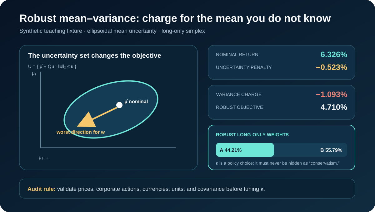
Ellipsoidal mean uncertainty and the portfolio's exposed direction

The portfolio does not care about every direction equally. Its worst direction is the one aligned against Q^T w.

From geometry to objective

For fixed weights, the weakest mean return is

min_(mu in U) mu^T w.

Substitute mu=mu_hat+Q u:

mu_hat^T w + min_(||u||<=kappa) u^T Q^T w.

The Euclidean norm's support function gives

mu_hat^T w-kappa||Q^T w||_2.

When the norm is nonzero, the adversarial direction is

u*=-kappa Q^T w/||Q^T w||_2.

That derivation is more important than the final penalty. It proves where the penalty came from. An arbitrary ridge term may be useful, but it is not this uncertainty set unless someone proves the connection.

The canonical optimizer maximizes

mu_hat^T w-kappa||Q^T w||_2-lambda w^T Sigma w

subject to non-negative weights summing to one. Covariance is fixed here. Joint mean/covariance uncertainty is a nearby but different problem.

Work through the numbers

Use this synthetic two-asset fixture:

Plain text

mu_hat = [0.08, 0.05]
Q = [[0.02, 0.00],
     [0.00, 0.01]]
kappa = 0.5
Sigma = [[0.04, 0.00],
         [0.00, 0.01]]
lambda = 1

At diagnostic weights [0.6,0.4], nominal return is 0.068. The uncertainty exposure is [0.012,0.004], with norm 0.0126491106. Half that norm is 0.0063245553, so robust return is 0.0616754447.

For the optimum, write w=[x,1-x]. The objective becomes

0.05+0.03x-0.005*sqrt(5x^2-2x+1)-0.04x^2-0.01(1-x)^2.

An independent bracketed derivative solve gives x=0.4421075077. At that point, robust return is 0.0580357014, variance is 0.0109308023, and the objective is 0.0471048991. The reference solver agrees within the declared tolerance.

The robust optimum does not have the largest nominal return. It chooses less exposure to the uncertain direction while still paying for covariance risk.

Radius is not confidence by itself

It is tempting to put a slider from 0% to 100% on kappa and call it confidence. That would be misleading. A statistical confidence interpretation requires a documented estimator, sampling assumptions, calibration procedure, and coverage argument. In this package, kappa is a model radius. The lab shows its sensitivity; it does not relabel it as a probability.

At kappa=0, the set collapses to the nominal mean and the uncertainty penalty vanishes. As kappa increases, the objective for any fixed candidate cannot increase. The optimized portfolio may change direction, so compare the full diagnostic—not just one weight.

Follow the calculation flow

Rendering system map…

The last box matters. A feasible portfolio is not automatically an optimum. The reference reports its projected-gradient norm and returns nonconverged if the stopping contract is not met.

Data errors are outside the ellipsoid

Robust optimization assumes its inputs mean what their labels say. It does not know that a price is pre-split while a quantity is post-split, that a cash dividend has been omitted from wealth, or that a Japanese-yen holding and a US- dollar holding were compared with inconsistent FX times. Those are data- contract failures, not small perturbations of the expected-return vector.

This is a lesson I learned from real portfolio systems: never let an optimizer be the first validator of historical holdings. Check instrument identity, units, price plausibility, corporate-action state, cash ledger, currency, observation time, and availability time before estimating mu_hat, Sigma, or Q. Otherwise the robust penalty may simply make corrupt inputs look calm.

Implementation walkthrough

The Python reference and TypeScript reference use deterministic projected gradient ascent. Each iteration computes nominal return, the norm penalty, variance, and gradient; backtracking prevents a step that lowers the objective; simplex projection restores long-only full investment.

The implementations require positive-definite covariance. The mathematical model can be expressed as a second-order cone program and can support broader production constraints, but an industrial solver must preserve status, residual, scale, and version information. Silent regularization changes the model and is not allowed.

Explore the uncertainty in the lab

The guided playground begins with the canonical optimum. Step from nominal mean to ellipsoid, exposed direction, worst-case mean, and final weights. Increase kappa to see the penalty and weights respond; set it to zero to run the nominal parity case; switch to the failure scenario to see indefinite covariance stop the calculation.

Ask one question at every stage: which input or rule caused the displayed change? If the answer is only “the optimizer did it,” the interface has not earned trust.

Tests and evidence boundaries

The test suite independently checks the diagnostic candidate, the scalar optimum, objective, robust return, and variance. It proves kappa=0 parity, penalty response, simplex invariants, invalid-radius rejection, covariance rejection, convergence status, and Python/TypeScript agreement.

The historical-example decision is deferred. A named case needs a licensed point-in-time panel and a defensible calibration of both Q and kappa. Without those, attaching a famous asset name to a synthetic ellipsoid would add false authority. Goldfarb and Iyengar support the general role of explicit parameter uncertainty and conic reformulations; the particular fixture and solver choices here are clearly labeled implementation decisions.

What this method does not promise

The true mean can fall outside the ellipsoid. Covariance can change even though we held it fixed. A one-period robust objective does not control path drawdown, liquidity, turnover, taxes, or funding. Stronger conservatism can also sacrifice useful return exposure. There is no universal best kappa.

Most importantly, robust does not mean profitable, safe, or correct. It means we optimized against one published uncertainty set and can audit the result.

Summary

Robust mean-variance becomes understandable when you can draw the uncertainty set, calculate Q^T w, identify the adversarial direction, and reproduce the norm penalty. The weight is the end of the evidence chain, not the evidence by itself.

Next, Distributionally Robust Portfolio moves from uncertainty about one mean vector to uncertainty about the probability distribution of returns.

Choose the family method by the decision you face

Your real question	Start with	What changes	What it does not solve
How should uncertain views modify a market prior?	Black-Litterman	Expected returns through a prior and views	Worst-case protection outside the view model
How unstable are optimized weights across plausible samples?	Resampled Efficient Frontier	Rows, replicate moments, and rank-matched frontiers	An explicit parameter guarantee
How should a bounded error in the mean affect allocation?	Robust Mean-Variance	Mean vector inside a declared ellipsoid	Errors outside the ellipsoid or changing covariance
Which portfolio ranks best under a declared distribution class and loss event?	Distributionally Robust Portfolio	The admissible return distribution	Universal or assumption-free safety
Which scenario mix maximizes long-run log growth?	Kelly Allocation	Objective and scenario wealth factors	A bounded mean-uncertainty policy

Related concepts and learning handoff

The reviewed The Fintech Builder chapter KKT checks and limits of an optimality claim (17:33–18:43) is a useful companion to the projected-gradient residual reported here. It is solver-QA context; it does not derive the ellipsoidal support function or choose kappa.

Workflows

Rendered from the canonical Mermaid sources linked by this article.

robust mean variance flow

Rendering system map…

ReferencesPrimary sources and evidence notes

Expand the source trail, evidence role, and limitations behind the engineering choices.

GI2003 — Robust Portfolio Selection Problems

Organization or authors: Donald Goldfarb and Garud Iyengar.
Source type: Original peer-reviewed research article, Mathematics of Operations Research.
Publication or effective date: 1 February 2003, 28(1), 1–38.
Version: DOI 10.1287/moor.28.1.1.14260.
URL or DOI: INFORMS record.
Accessed: 2026-09-15.
Jurisdiction: None; mathematical portfolio methodology.
Supports: Explicit uncertainty structures for market parameters and tractable second-order-cone reformulations.
Limitations: The package uses a transparent mean-only ellipsoidal specialization, not every model in the paper.

TK2004 — A Robust Portfolio Selection Approach

Organization or authors: Recep Tütüncü and Mark Koenig.
Source type: Peer-reviewed Annals of Operations Research article and author manuscript.
Publication or effective date: 2004, 132, 157–187.
Version: DOI 10.1023/B:ANOR.0000045281.41041.ed.
URL or DOI: Author PDF.
Accessed: 2026-09-15.
Jurisdiction: None.
Supports: Robust portfolio selection as optimization against parameter uncertainty.
Limitations: Does not make this package's Q or kappa a universal calibration.

MOSEK-ROBUST — Estimation error and robust optimization

Organization or authors: MOSEK ApS.
Source type: Maintained official technical documentation.
Publication or effective date: Online edition accessed 2026-09-15.
Version: Portfolio Optimization Cookbook.
URL or DOI: Estimation error chapter.
Accessed: 2026-09-15.
Jurisdiction: None.
Supports: Distinction between robust estimation, Bayesian methods, resampling, and robust optimization.
Limitations: Vendor documentation does not replace the original research sources.

Implementation

Full dependency-light reference implementations in both supported languages.

robust-mean-variance.ts

export class ContractError extends Error {}

type Vector = number[];
type Matrix = number[][];

const dot = (a: Vector, b: Vector): number => a.reduce((sum, x, i) => sum + x * b[i], 0);
const matrixVector = (matrix: Matrix, vector: Vector): Vector => matrix.map((row) => dot(row, vector));
const norm = (vector: Vector): number => Math.sqrt(dot(vector, vector));

function projectSimplex(vector: Vector): Vector {
  const sorted = [...vector].sort((a, b) => b - a);
  let cumulative = 0;
  let rho = -1;
  sorted.forEach((value, index) => {
    cumulative += value;
    if (value - (cumulative - 1) / (index + 1) > 0) rho = index;
  });
  const theta = (sorted.slice(0, rho + 1).reduce((a, b) => a + b, 0) - 1) / (rho + 1);
  return vector.map((value) => Math.max(value - theta, 0));
}

function validateInputs(mean: Vector, covariance: Matrix, uncertaintyShape: Matrix): [Vector, Matrix, Matrix] {
  const mu = mean.map(Number);
  const n = mu.length;
  const sigma = covariance.map((row) => row.map(Number));
  const shape = uncertaintyShape.map((row) => row.map(Number));

  if (!n || mu.some((value) => !Number.isFinite(value))) {
    throw new ContractError("mean must be finite");
  }
  if (
    sigma.length !== n ||
    sigma.some((row) => row.length !== n) ||
    sigma.flat().some((value) => !Number.isFinite(value))
  ) {
    throw new ContractError("covariance shape/values invalid");
  }
  if (sigma.some((row, i) => row.some((value, j) => Math.abs(value - sigma[j][i]) > 1e-12))) {
    throw new ContractError("covariance must be symmetric");
  }
  if (
    shape.length !== n ||
    !shape[0]?.length ||
    shape.some((row) => row.length !== shape[0].length) ||
    shape.flat().some((value) => !Number.isFinite(value))
  ) {
    throw new ContractError("uncertainty shape Q must be finite n by m");
  }

  const cholesky = Array.from({ length: n }, () => Array(n).fill(0));
  for (let i = 0; i < n; i += 1) {
    for (let j = 0; j <= i; j += 1) {
      const correction = Array.from(
        { length: j },
        (_, k) => cholesky[i][k] * cholesky[j][k],
      ).reduce((a, b) => a + b, 0);
      const residual = sigma[i][j] - correction;
      if (i === j) {
        if (residual <= 1e-14) throw new ContractError("covariance must be positive definite");
        cholesky[i][j] = Math.sqrt(residual);
      } else {
        cholesky[i][j] = residual / cholesky[j][j];
      }
    }
  }
  return [mu, sigma, shape];
}

export interface RobustResult {
  weights: Vector;
  nominalReturn: number;
  uncertaintyPenalty: number;
  robustReturn: number;
  variance: number;
  objective: number;
  worstCaseMean: Vector;
  iterations: number;
  projectedGradientNorm: number;
  status: "optimal" | "nonconverged";
}

export function robustMeanVariance(
  mean: Vector,
  covariance: Matrix,
  uncertaintyShape: Matrix,
  kappa: number,
  riskPenalty = 1,
  maxIterations = 20_000,
  tolerance = 2e-9,
): RobustResult {
  const [mu, sigma, shape] = validateInputs(mean, covariance, uncertaintyShape);
  const n = mu.length;
  const m = shape[0].length;

  if (!Number.isFinite(kappa) || kappa < 0) {
    throw new ContractError("kappa must be finite and non-negative");
  }
  if (!(riskPenalty > 0) || maxIterations < 1 || !(tolerance > 0)) {
    throw new ContractError("solver controls are invalid");
  }

  const terms = (weights: Vector) => {
    const qTransposeWeights = Array.from(
      { length: m },
      (_, j) => shape.reduce((sum, row, i) => sum + row[j] * weights[i], 0),
    );
    const qNorm = norm(qTransposeWeights);
    const variance = dot(weights, matrixVector(sigma, weights));
    const penalty = kappa * qNorm;
    return {
      objective: dot(mu, weights) - penalty - riskPenalty * variance,
      qTransposeWeights,
      qNorm,
      variance,
      penalty,
    };
  };

  const gradient = (weights: Vector, state: ReturnType<typeof terms>): Vector => {
    const risk = matrixVector(sigma, weights);
    const uncertainty = state.qNorm <= 1e-18
      ? Array(n).fill(0)
      : shape.map((row) => kappa * dot(row, state.qTransposeWeights) / state.qNorm);
    return mu.map((value, i) => value - uncertainty[i] - 2 * riskPenalty * risk[i]);
  };

  let weights = Array(n).fill(1 / n);
  let state = terms(weights);
  let iteration = 0;
  let projectedGradientNorm = Infinity;
  for (iteration = 1; iteration <= maxIterations; iteration += 1) {
    const currentGradient = gradient(weights, state);
    const mapped = projectSimplex(weights.map((value, i) => value + currentGradient[i]));
    projectedGradientNorm = norm(mapped.map((value, i) => value - weights[i]));
    if (projectedGradientNorm <= tolerance) break;

    let step = 1;
    let accepted = false;
    while (step >= 1e-14) {
      const candidate = projectSimplex(weights.map((value, i) => value + step * currentGradient[i]));
      const nextState = terms(candidate);
      const displacement = candidate.map((value, i) => value - weights[i]);
      if (nextState.objective >= state.objective + 1e-4 * dot(currentGradient, displacement)) {
        weights = candidate;
        state = nextState;
        accepted = true;
        break;
      }
      step *= 0.5;
    }
    if (!accepted) break;
  }

  const finalGradient = gradient(weights, state);
  projectedGradientNorm = norm(
    projectSimplex(weights.map((value, i) => value + finalGradient[i]))
      .map((value, i) => value - weights[i]),
  );
  const direction = state.qNorm <= 1e-18
    ? Array(m).fill(0)
    : state.qTransposeWeights.map((value) => -kappa * value / state.qNorm);
  const worstCaseMean = mu.map((value, i) => value + dot(shape[i], direction));

  return {
    weights,
    nominalReturn: dot(mu, weights),
    uncertaintyPenalty: state.penalty,
    robustReturn: dot(mu, weights) - state.penalty,
    variance: state.variance,
    objective: state.objective,
    worstCaseMean,
    iterations: Math.min(iteration, maxIterations),
    projectedGradientNorm,
    status: projectedGradientNorm <= tolerance ? "optimal" : "nonconverged",
  };
}

Playground

The embedded lab now expands to its full document height, keeping the article as the only scroll surface.

Full-height labplaygroundOpen full screen

Written by

Islam Baraka

Fintech engineer building market-data and financial systems, and the author of every article, glossary record, and reference implementation on The Fintech Builder.