
 By Islam Baraka
Kelly is often introduced with one favorable coin toss and one compact betting formula. That example is useful history, but it can leave portfolio builders with the wrong mental model. Real allocation involves several assets, several possible outcomes, and a strict question in every outcome: is the next wealth factor still positive?
This tutorial builds the general finite-scenario version. We will calculate probability-weighted log growth, solve a long-only multi-asset allocation, inspect every scenario wealth factor, and scale full Kelly into explicit cash. We will not call the result safe, and we will not hide zero wealth behind a small numerical epsilon.
Why logarithmic wealth changes the decision
An arithmetic-return maximizer likes the largest expected payoff. It does not care enough about a rare outcome that destroys the bankroll. Kelly maximizes
G(w)=sum_s p_s log(1+w^T r_s).
Here r_s is the vector of simple returns in scenario s, p_s is its
probability, and w is the portfolio. The factor 1+w^T r_s is wealth after
the scenario divided by wealth before it.
The logarithm converts multiplication across repeated periods into addition and makes zero wealth an absolute boundary. That creates the growth-optimal logic under the supplied model. It does not create a reliable model of the future.
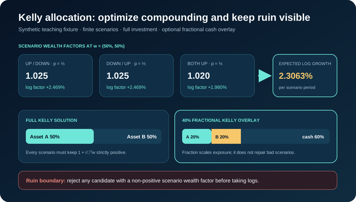
The visual keeps the individual factors visible. An average can look healthy while one factor approaches zero and dominates the log objective.
The canonical contract
We choose w>=0 with 1^T w=1 and require
1+w^T r_s>0
for every scenario. The return inputs are decimal simple returns. If a data source supplies log returns, transform the model intentionally; do not insert them into the simple-return wealth equation.
A return of -1 means that asset loses 100%. It is valid input, but a candidate
fully allocated to that asset produces a zero wealth factor and is outside the
log domain. A simple return below -1 is invalid. If every asset is at -1 in
the same scenario, full investment has no feasible solution.
The finite-scenario gradient is
dG/dw_j=sum_s p_s r_(s,j)/(1+w^T r_s).
Because log is concave, G is concave on the positive domain. The reference
solver uses projected gradient ascent with backtracking and publishes its
projected-gradient residual.
A symmetric example with an exact answer
Use three synthetic, equally likely scenarios:
| Scenario | Asset A | Asset B |
|---|---|---|
| A leads | 10% | -5% |
| B leads | -5% | 10% |
| Both gain | 2% | 2% |
At equal weights, the factors are [1.025,1.025,1.02]. Therefore
G=(2 log(1.025)+log(1.02))/3=0.02306261749.
At [1,0], the factors are [1.10,0.95,1.02] and
G=0.02127317090. Concentration has a slightly larger best outcome, but the
weaker second factor reduces geometric growth.
We can prove the optimum without trusting code. Write w=[x,1-x]. The first
two factors are 0.95+0.15x and 1.10-0.15x. They are symmetric around
x=0.5, and their sum is fixed. Strict concavity of the log sum makes
x=0.5 the unique optimum.
Fractional Kelly must leave visible cash
Suppose the full Kelly risky weights are [0.5,0.5], but the policy selects a
40% fraction. The correct output is risky weights [0.2,0.2] and cash weight
0.6. If a system scales the risky weights and then renormalizes them back to
[0.5,0.5], it has undone the fraction.
Cash is not an invisible remainder. Its return convention, currency, funding rules, and whether it can be negative all belong in a production contract. The helper here assumes a zero-return cash sleeve only to demonstrate the arithmetic.
Why scenario quality is the real risk
Kelly can be aggressively correct about an incomplete model. If a severe loss scenario is missing or assigned too little probability, the optimizer may take more risk precisely because the logarithmic objective sees no reason not to.
Data lineage is therefore part of the allocation. Before constructing returns, verify security identity, split state, cash dividends, quantity units, quote currency, and FX time. I have encountered old portfolio records where these items were mixed and the apparent return never existed economically. If a cash dividend is paid but only the price drop is recorded, the wealth factor is wrong. If a pre-split price meets a post-split quantity, the factor is wrong. Kelly cannot infer the missing ledger event.
Probabilities also need provenance. Equal weights can describe an empirical sample; they do not become true outcome probabilities merely because the code accepts them. A forecasting or scenario-generation model should record its knowledge cutoff, version, calibration, and uncertainty separately.
Implementation walkthrough
The Python implementation and TypeScript implementation share the same validation, simplex projection, gradient, backtracking, and stopping rule. The result includes the full vector of wealth factors and its minimum, not only the final weights.
The solver starts at equal weight. Because all valid asset returns are at least
-1, equal weight is positive in a scenario whenever at least one asset is
above -1. A scenario where every asset is exactly -1 is rejected as
infeasible before iteration.
Backtracking prevents a step from leaving the positive domain or lowering the
objective. If the projected-gradient residual does not meet tolerance, the
status is nonconverged. A feasible portfolio is not silently upgraded to an
optimum.
Explore full, fractional, and failure states
Open the Kelly guided playground. The canonical state shows all three factors and the equal-weight optimum. Step through factor calculation, logarithms, probability weighting, and the optimizer. Move the fraction control and watch risky weights shrink while cash grows. The failure scenario places all assets at a 100% loss in one outcome and shows why the fully invested problem has no positive-domain solution.
What to notice: the minimum factor is as important as expected log growth. A result that does not expose its weakest scenario is difficult to review.
Tests that protect the definition
The shared fixture verifies the exact equal-weight objective and the
concentrated endpoint. Scenario rows and their probabilities can be permuted
together without changing the solution. Fractional Kelly must preserve the
declared cash weight. Candidate evaluation rejects zero wealth, the optimizer
rejects an all-ruin scenario, and simple returns below -1 fail input validation.
Python and TypeScript reproduce the same result.
These tests prove the calculation, not the probability model. They do not show that the scenarios are exhaustive or that the allocation has acceptable drawdown.
Kelly, drawdown, and suitability
The original Kelly result is about asymptotic growth under its assumptions. Finite-horizon investors can experience deep drawdowns before that asymptotic logic becomes comforting. Risk-constrained Kelly adds an explicit drawdown- probability control. Fractional Kelly is a simpler heuristic. Both are distinct from full Kelly and should be labeled.
The historical-example decision is deferred. A named market example needs licensed scenario returns, defensible probabilities, point-in-time availability, and policies for costs, cash, leverage, drawdown, taxes, and rebalancing. Without those, backfilled Kelly weights would invite hindsight.
What full Kelly does not promise
It does not promise positive realized return, small drawdown, low volatility, liquidity, tax efficiency, or suitability. It assumes the supplied outcome model and one-period mapping are meaningful. Dependence over time, changing probabilities, fat tails outside the scenario set, execution costs, and funding constraints can materially alter the decision.
This tutorial is educational. It is not investment advice, and the synthetic weights are not recommendations.
Summary
An auditable Kelly allocation exposes the complete chain: simple-return scenarios, probabilities, candidate weights, every wealth factor, expected log growth, convergence residual, and explicit cash for any fractional scale. The logarithm makes ruin impossible to hide mathematically; our implementation and interface should not hide it operationally either.
Kelly completes this family by changing the objective. Black-Litterman changes the mean through views, REF measures sampling instability, robust mean-variance protects against a parameter set, and DRO protects against a distribution class.
Choose the family method by the decision you face
| Your real question | Start with | What changes | What it does not solve |
|---|---|---|---|
| How should uncertain views modify a market prior? | Black-Litterman | Expected returns through a prior and views | Long-run growth under supplied scenarios |
| How unstable are optimized weights across plausible samples? | Resampled Efficient Frontier | Rows, replicate moments, and rank-matched frontiers | Ruin avoidance outside observed samples |
| How should a bounded error in the mean affect allocation? | Robust Mean-Variance | Mean vector inside a declared ellipsoid | Log-wealth optimization |
| Which portfolio ranks best under a declared distribution class and loss event? | Distributionally Robust Portfolio | The admissible return distribution | Scenario-specific compounding |
| Which scenario mix maximizes long-run log growth? | Kelly Allocation | Objective and scenario wealth factors | Drawdown comfort, suitability, or scenario quality |
Related concepts and learning handoff
The reviewed The Fintech Builder chapter KKT checks and limits of an optimality claim (17:33–18:43) helps review simplex feasibility and first-order optimality after the log-growth solve. It does not justify the scenario probabilities or prove that full Kelly is suitable for a person.
Rendered from the canonical Mermaid sources linked by this article.
kelly allocation flow
ReferencesPrimary sources and evidence notesExpand the source trail, evidence role, and limitations behind the engineering choices.
Expand the source trail, evidence role, and limitations behind the engineering choices.
KELLY1956 — A New Interpretation of Information Rate
- Organization or authors: J. L. Kelly Jr.
- Source type: Original peer-reviewed Bell System Technical Journal article.
- Publication or effective date: July 1956, 35(4), 917–926.
- Version: DOI
10.1002/j.1538-7305.1956.tb03809.x. - URL or DOI: Wiley record.
- Accessed: 2026-09-15.
- Jurisdiction: None; information-theoretic and gambling framework.
- Supports: Maximum exponential growth-rate interpretation and arbitrary-odds extension.
- Limitations: It is not a portfolio data contract, drawdown prescription, tax model, or profitability forecast.
BRB2016 — Risk-Constrained Kelly Gambling
- Organization or authors: Enzo Busseti, Ernest K. Ryu, and Stephen Boyd.
- Source type: Peer-reviewed Journal of Investing paper and author manuscript.
- Publication or effective date: Fall 2016, 25(3), 118–134.
- Version: Author manuscript dated 19 March 2016.
- URL or DOI: Stanford paper and code page.
- Accessed: 2026-09-15.
- Jurisdiction: None.
- Supports: General finite-outcome Kelly formulation, explicit probabilities and non-negative gross payoffs, and the distinction between drawdown-constrained and fractional approaches.
- Limitations: The risk-constrained extension is a comparison, not part of the canonical objective.
SB2018 — Distributional Robust Kelly Gambling
- Organization or authors: Qingyun Sun and Stephen Boyd.
- Source type: Original research manuscript.
- Publication or effective date: December 2018.
- Version: arXiv
1812.10371. - URL or DOI: Stanford record.
- Accessed: 2026-09-15.
- Jurisdiction: None.
- Supports: Distributionally robust Kelly as a distinct finite-outcome extension when probabilities are uncertain.
- Limitations: That ambiguity-set problem is not implemented here and must not be conflated with ordinary Kelly.
Full dependency-light reference implementations in both supported languages.
export class ContractError extends Error{};type V=number[];type M=number[][];const dot=(a:V,b:V)=>a.reduce((s,x,i)=>s+x*b[i],0),norm=(x:V)=>Math.sqrt(dot(x,x));
function simplex(v:V):V{const u=[...v].sort((a,b)=>b-a);let s=0,rho=-1;u.forEach((x,i)=>{s+=x;if(x-(s-1)/(i+1)>0)rho=i});const theta=(u.slice(0,rho+1).reduce((a,b)=>a+b,0)-1)/(rho+1);return v.map(x=>Math.max(x-theta,0));}
export function logGrowth(weights:V,returns:M,probabilities:V):number{const w=weights.map(Number),rows=returns.map(r=>r.map(Number)),p=probabilities.map(Number);if(!w.length||w.some(x=>x<0||!Number.isFinite(x))||Math.abs(w.reduce((a,b)=>a+b,0)-1)>1e-10)throw new ContractError("weights must be a finite simplex vector");if(rows.length!==p.length||!rows.length||rows.some(r=>r.length!==w.length))throw new ContractError("return scenario shape mismatch");const f=rows.map(r=>1+dot(w,r));if(Math.min(...f)<=0)throw new ContractError("all scenario wealth factors must be strictly positive");return p.reduce((s,x,i)=>s+x*Math.log(f[i]),0)}
export interface KellyResult{weights:V;expectedLogGrowth:number;wealthFactors:V;minimumWealthFactor:number;arithmeticExpectedReturn:number;iterations:number;projectedGradientNorm:number;status:"optimal"|"nonconverged"}
export function kellyAllocation(returns:M,probabilities?:V,maxIterations=30000,tolerance=1e-12):KellyResult{const rows=returns.map(r=>r.map(Number));if(!rows.length||!rows[0]?.length||rows.some(r=>r.length!==rows[0].length)||rows.flat().some(x=>!Number.isFinite(x)))throw new ContractError("returns must be a finite rectangular matrix");if(rows.flat().some(x=>x<-1))throw new ContractError("simple returns below -1 are invalid");const t=rows.length,n=rows[0].length,p=probabilities?.map(Number)??Array(t).fill(1/t);if(p.length!==t||p.some(x=>x<0||!Number.isFinite(x))||Math.abs(p.reduce((a,b)=>a+b,0)-1)>1e-10)throw new ContractError("probabilities must be a finite simplex vector");if(rows.some(r=>Math.max(...r)<=-1))throw new ContractError("no simplex portfolio has positive wealth in every scenario");if(maxIterations<1||!(tolerance>0))throw new ContractError("iteration controls invalid");const terms=(w:V)=>{const factors=rows.map(r=>1+dot(w,r));return{objective:Math.min(...factors)<=0?-Infinity:p.reduce((s,x,i)=>s+x*Math.log(factors[i]),0),factors}},grad=(w:V,f:V)=>Array.from({length:n},(_,j)=>p.reduce((sum,x,s)=>sum+x*rows[s][j]/f[s],0));let w=Array(n).fill(1/n),z=terms(w),iteration=0,pg=Infinity;for(iteration=1;iteration<=maxIterations;iteration++){const g=grad(w,z.factors),mapped=simplex(w.map((x,i)=>x+g[i]));pg=norm(mapped.map((x,i)=>x-w[i]));if(pg<=tolerance)break;let step=1,accepted=false;while(step>=1e-14){const candidate=simplex(w.map((x,i)=>x+step*g[i])),nz=terms(candidate);if(nz.objective>=z.objective+1e-4*dot(g,candidate.map((x,i)=>x-w[i]))){w=candidate;z=nz;accepted=true;break}step*=.5}if(!accepted)break}const g=grad(w,z.factors);pg=norm(simplex(w.map((x,i)=>x+g[i])).map((x,i)=>x-w[i]));return{weights:w,expectedLogGrowth:z.objective,wealthFactors:z.factors,minimumWealthFactor:Math.min(...z.factors),arithmeticExpectedReturn:p.reduce((s,x,i)=>s+x*dot(w,rows[i]),0),iterations:Math.min(iteration,maxIterations),projectedGradientNorm:pg,status:pg<=Math.max(tolerance,1e-9)?"optimal":"nonconverged"}}
export function fractionalKelly(fullWeights:V,fraction:number):{riskyWeights:V,cashWeight:number}{if(!Number.isFinite(fraction)||fraction<0||fraction>1)throw new ContractError("fraction must lie in [0,1]");if(fullWeights.some(x=>x<0)||Math.abs(fullWeights.reduce((a,b)=>a+b,0)-1)>1e-10)throw new ContractError("full weights must be a simplex vector");return{riskyWeights:fullWeights.map(x=>fraction*x),cashWeight:1-fraction}}
The embedded lab now expands to its full document height, keeping the article as the only scroll surface.