D14-F03-A01 / Released engineering topic

Black-Litterman: Turn Market Weights and Uncertain Views into Auditable Allocations

A production-minded guide to Black-Litterman.

By Islam Baraka 8 min read Reviewed Sep 15, 2026 Updated Sep 15, 2026 Python + TypeScript

Black-Litterman: Turn Market Weights and Uncertain Views into Auditable Allocations

D14 / D14-F03

When somebody shows me a portfolio optimizer, I do not begin by admiring the weights. I ask where the expected returns came from. That question matters because a mean-variance optimizer can turn a tiny, noisy return difference into a very large position. The calculation may be flawless while the premise is fragile.

Black-Litterman gives us a better starting conversation. Instead of treating a historical sample mean as truth, we begin with returns implied by a supplied market portfolio. Then we express investor views as equations and state how uncertain those equations are. The result is a posterior mean that can feed a separate portfolio optimizer.

In this tutorial we will reproduce that chain completely: equilibrium prior, relative view, uncertainty-weighted update, and long-only allocation. More important, we will keep the boundaries visible. A posterior is not a fact, a confidence control is not automatically a probability, and sophisticated matrix algebra cannot repair impossible historical prices.

The practical question

Suppose the reference market holds two assets at 50% each. You believe asset A will outperform asset B by four percentage points over the modeled period, but you do not want one view to erase the information in the market portfolio. Black-Litterman asks: how far should the expected returns move from the neutral prior when the view carries a declared error variance?

That is already more disciplined than typing two return forecasts into an optimizer. It forces three separate decisions:

What portfolio and covariance define the prior?
What exactly does the view say?
How uncertain is the view relative to the prior?

The final position limits are a fourth decision. Black-Litterman does not make them for us.

Intuition before notation

Think of the prior as an anchor, the view as a directional pull, and Omega as the amount of slack in the rope. A precise view pulls harder. An uncertain view allows the posterior to stay near the anchor. If the view exactly matches the prior, there is no pull at all.

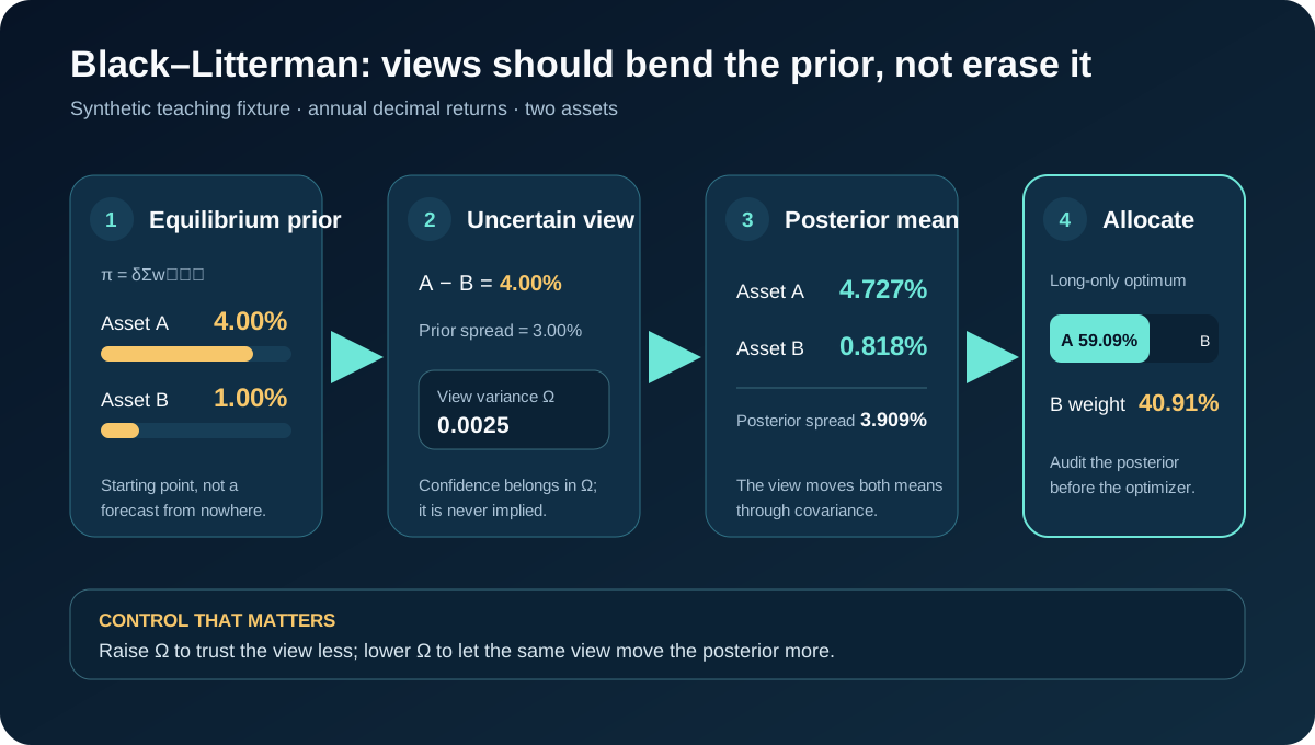
Black-Litterman prior, view and allocation bridge

The visual separates the posterior engine from the allocation engine. This is not cosmetic. Many implementation disagreements arise because one system updates only the mean, another also updates covariance, and a third silently changes constraints. Here we freeze one version and name everything else.

The canonical contract

Let w_mkt be non-negative market weights summing to one, Sigma a positive- definite covariance matrix, and delta>0 the risk-aversion coefficient used for reverse optimization. The implied equilibrium excess return is

Pi = delta Sigma w_mkt.

Let P contain the linear views. A row [1,-1] means asset A minus asset B. Let q contain the target return for each row, Omega the positive-definite view-error covariance, and tau>0 the prior uncertainty scale. The posterior mean is

mu_BL = Pi + tau Sigma P^T(P tau Sigma P^T + Omega)^-1(q-P Pi).

The expression q-P Pi is the surprise. If it is zero, the posterior equals the prior. The implementation solves the middle linear system; it does not form a numerical inverse.

This package then solves

maximize mu_BL^T w - lambda w^T Sigma w

subject to w>=0 and 1^T w=1. We retain Sigma for this stage. Updating the posterior covariance is a valid nearby choice, but it is not this package's choice.

A worked two-asset example

All values below are synthetic decimal returns for one consistent period:

Plain text

w_mkt = [0.5, 0.5]
Sigma = [[0.04, 0.00],
         [0.00, 0.01]]
delta = 2
tau = 0.5
P = [[1, -1]]
q = [0.04]
Omega = [[0.0025]]
lambda = 1

The prior is Pi=[0.04,0.01], so the prior already implies a 3% relative view. Our target is 4%; the surprise is 1%.

The prior-scaled loading is [0.02,-0.005]. The scalar view system is 0.0275. Multiplying the loading by 0.01/0.0275 gives the update [0.0072727273,-0.0018181818]. Therefore:

Plain text

mu_BL = [0.0472727273, 0.0081818182]

Notice what did not happen: the posterior relative return did not jump blindly to the view. It moved according to the covariance, tau, and Omega.

For the long-only allocation, write w=[x,1-x]. Differentiating the quadratic objective gives x=0.5909090909. The final weights are [0.5909090909,0.4090909091], and the independently calculated objective is 0.0156404959.

Now change q from 0.04 to 0.03. The surprise becomes zero, so the posterior returns exactly to Pi. That identity is one of the strongest simple tests in the package.

The input lesson I would not skip

I have seen portfolio records where a price did not match any plausible historical market state, pre- and post-split units were mixed, cash dividends looked like losses, and holdings in several currencies were compared before a consistent FX translation. A Bayesian label does not protect us from those mistakes. It can make them look more sophisticated.

The core function therefore starts after a provenance adapter. That adapter must establish instrument identity, period, observation and availability time, split and dividend basis, quote currency, FX direction and timestamp, missing- value policy, and stable asset order. If a source price is impossible for the date, fail the input. Do not let a posterior average legitimize it.

Read the data flow, not only the formula

Rendering system map…

The calculation flow provides natural review checkpoints. We can inspect the prior before debating the view, inspect the posterior before applying constraints, and inspect feasibility before publishing weights.

Implementation walkthrough

The Python reference and TypeScript reference use the same operations and shared fixture. Each validates dimensions and positive definiteness, solves the view system with pivoting, computes the posterior, and enumerates active asset subsets for the small long-only quadratic program.

Enumeration is useful here because it makes the teaching oracle inspectable. It is exponential, so the code refuses universes larger than 12 assets. A production system should use a mature quadratic solver, preserve raw status and residuals, and never replace an infeasible result with equal weights.

Use the guided lab

Open the Black-Litterman guided playground. Start with the canonical relative view, then step through the prior, surprise, posterior, and allocation. Increase Omega and watch the tilt shrink. Switch to the neutral view and confirm that the update disappears. The failure scenario shows why zero view variance is rejected instead of treated as “perfect confidence.”

The important observation is not simply that weights change. It is why: the view surprise and its declared uncertainty change first, then the posterior, then the constrained allocation.

Tests that earn trust

The shared fixture checks posterior returns to tight tolerance and reproduces the independent one-variable optimum. Additional tests prove the neutral-view identity, the weakening effect of larger Omega, simplex invariants, singular view-covariance rejection, indefinite covariance rejection, and Python/ TypeScript parity.

Those tests establish implementation correctness for the selected contract. They do not validate the economic quality of a view or establish future performance.

Where Black-Litterman stops

Black-Litterman does not tell us how to forecast q, calibrate Omega, select tau, estimate Sigma, or decide whether market capitalization is the right prior. It does not model turnover, taxes, liquidity, leverage, drawdown, or multi-period learning here. It also does not become robust optimization merely because it responds smoothly to uncertainty.

The historical-example decision is deferred. A real case needs licensed point-in-time market weights, covariance and return horizons, view formation and knowledge time, currency and corporate-action basis, and the actual constraints. Without those facts, a famous market story would make the article less reproducible, not more.

Summary

An auditable Black-Litterman implementation has three visible layers: implied equilibrium prior, uncertainty-weighted view update, and separately declared allocation. If you can reproduce Pi, q-P Pi, the posterior, and the final objective from one fixture, you can review the system rather than trust its label.

Next, Resampled Efficient Frontier asks a different question: how stable is an optimizer when we rebuild it on many resampled versions of the input rows?

Choose the family method by the decision you face

Your real question	Start with	What changes	What it does not solve
How should uncertain views modify a market prior?	Black-Litterman	Expected returns through `P`, `q`, `Omega`, and `tau`	Whether the views are true
How unstable are optimized weights across plausible samples?	Resampled Efficient Frontier	Rows, replicate moments, and rank-matched frontiers	Structural errors repeated in every sample
How should a bounded error in the mean affect allocation?	Robust Mean-Variance	Mean vector inside a declared ellipsoid	Distribution shift outside that set
Which portfolio ranks best under a declared distribution class and loss event?	Distributionally Robust Portfolio	The admissible return distribution	Universal or assumption-free safety
Which scenario mix maximizes long-run log growth?	Kelly Allocation	Objective and scenario wealth factors	Drawdown comfort or scenario quality

Related concepts and learning handoff

The reviewed The Fintech Builder chapter KKT checks and limits of an optimality claim (17:33–18:43) is useful after the allocation step: it explains why feasibility and stationarity checks belong beside an optimizer result. It is supporting solver-quality material, not a derivation of the Black-Litterman posterior.

Workflows

Rendered from the canonical Mermaid sources linked by this article.

black litterman flow

Rendering system map…

ReferencesPrimary sources and evidence notes

Expand the source trail, evidence role, and limitations behind the engineering choices.

BL1992 — Global Portfolio Optimization

Organization or authors: Fischer Black and Robert Litterman.
Source type: Original practitioner research article, Financial Analysts Journal.
Publication or effective date: 1 September 1992, 48(5), 28–43.
Version: DOI 10.2469/faj.v48.n5.28.
URL or DOI: CFA Institute record.
Accessed: 2026-09-15.
Jurisdiction: Global portfolio methodology; not regulatory guidance.
Supports: Equilibrium excess returns as a neutral starting point, absolute/relative views, and confidence-weighted tilts.
Limitations: The landing record does not make later tau, Omega, posterior-covariance, or constraint conventions universal.

MOSEK-EST — Estimation error and Bayesian allocation

Organization or authors: MOSEK ApS.
Source type: Maintained official technical documentation.
Publication or effective date: Online edition accessed 2026-09-15.
Version: Portfolio Optimization Cookbook, estimationerror.html.
URL or DOI: Estimation error chapter.
Accessed: 2026-09-15.
Jurisdiction: None; solver and modeling documentation.
Supports: Sensitivity of mean-variance optimization, a Black-Litterman prior/view setup, and distinctions from robust optimization.
Limitations: Vendor documentation is explanatory evidence, not the original definition or a universal default policy.

Implementation

Full dependency-light reference implementations in both supported languages.

black-litterman.ts

export class ContractError extends Error {}
type Vector = number[];
type Matrix = number[][];

function finiteVector(values: number[], name: string): Vector {
  const out = values.map(Number);
  if (!out.length || out.some((x) => !Number.isFinite(x))) throw new ContractError(`${name} must be a non-empty finite vector`);
  return out;
}
function matrix(values: number[][], rows: number, cols: number, name: string): Matrix {
  const out = values.map((row) => row.map(Number));
  if (out.length !== rows || out.some((row) => row.length !== cols) || out.flat().some((x) => !Number.isFinite(x))) {
    throw new ContractError(`${name} must have shape ${rows}x${cols} with finite values`);
  }
  return out;
}
function solve(a: Matrix, b: Vector): Vector {
  const n = b.length;
  const aug = a.map((row, i) => [...row, b[i]]);
  for (let col = 0; col < n; col++) {
    let pivot = col;
    for (let row = col + 1; row < n; row++) if (Math.abs(aug[row][col]) > Math.abs(aug[pivot][col])) pivot = row;
    if (Math.abs(aug[pivot][col]) <= 1e-14) throw new ContractError("linear system is singular");
    [aug[col], aug[pivot]] = [aug[pivot], aug[col]];
    const scale = aug[col][col];
    aug[col] = aug[col].map((x) => x / scale);
    for (let row = 0; row < n; row++) if (row !== col) {
      const factor = aug[row][col];
      aug[row] = aug[row].map((x, j) => x - factor * aug[col][j]);
    }
  }
  return aug.map((row) => row[n]);
}
function validateSpd(a: Matrix, name: string): void {
  const n = a.length;
  if (a.some((row, i) => row.some((x, j) => Math.abs(x - a[j][i]) > 1e-12))) throw new ContractError(`${name} must be symmetric`);
  const lower = Array.from({ length: n }, () => Array(n).fill(0));
  for (let i = 0; i < n; i++) for (let j = 0; j <= i; j++) {
    const value = a[i][j] - Array.from({ length: j }, (_, k) => lower[i][k] * lower[j][k]).reduce((x, y) => x + y, 0);
    if (i === j) {
      if (value <= 1e-14) throw new ContractError(`${name} must be symmetric positive definite`);
      lower[i][j] = Math.sqrt(value);
    } else lower[i][j] = value / lower[j][j];
  }
}
const dot = (a: Vector, b: Vector) => a.reduce((sum, x, i) => sum + x * b[i], 0);
const matVec = (a: Matrix, x: Vector) => a.map((row) => dot(row, x));
function* combinations(n: number, k: number, start = 0, prefix: number[] = []): Generator<number[]> {
  if (prefix.length === k) { yield prefix; return; }
  for (let i = start; i < n; i++) yield* combinations(n, k, i + 1, [...prefix, i]);
}
function longOnlyQp(mu: Vector, sigma: Matrix, riskPenalty: number): Vector {
  const n = mu.length;
  if (n > 12) throw new ContractError("reference active-set allocator supports at most 12 assets");
  let best: { objective: number; weights: Vector } | undefined;
  for (let size = 1; size <= n; size++) for (const active of combinations(n, size)) {
    let weights = Array(n).fill(0);
    if (size === 1) weights[active[0]] = 1;
    else {
      const sub = active.map((i) => active.map((j) => sigma[i][j]));
      let invMu: Vector, invOne: Vector;
      try { invMu = solve(sub, active.map((i) => mu[i])); invOne = solve(sub, Array(size).fill(1)); } catch { continue; }
      const lagrange = (invMu.reduce((a, b) => a + b, 0) - 2 * riskPenalty) / invOne.reduce((a, b) => a + b, 0);
      const subW = invMu.map((x, i) => (x - lagrange * invOne[i]) / (2 * riskPenalty));
      if (Math.min(...subW) <= 1e-12) continue;
      active.forEach((asset, i) => { weights[asset] = subW[i]; });
    }
    const variance = dot(weights, matVec(sigma, weights));
    const objective = dot(mu, weights) - riskPenalty * variance;
    if (!best || objective > best.objective + 1e-14) best = { objective, weights };
  }
  if (!best) throw new ContractError("no feasible simplex allocation");
  return best.weights;
}

export interface BlackLittermanInput {
  marketWeights: number[]; covariance: number[][]; riskAversion: number; tau: number;
  viewMatrix: number[][]; viewReturns: number[]; viewErrorCovariance: number[][]; riskPenalty?: number;
}
export interface BlackLittermanResult {
  priorReturns: Vector; posteriorReturns: Vector; weights: Vector; priorView: Vector;
  posteriorView: Vector; viewSurprise: Vector; variance: number; objective: number; status: "optimal";
}
export function blackLittermanAllocate(input: BlackLittermanInput): BlackLittermanResult {
  const wm = finiteVector(input.marketWeights, "marketWeights");
  const n = wm.length;
  if (wm.some((x) => x < 0) || Math.abs(wm.reduce((a, b) => a + b, 0) - 1) > 1e-10) throw new ContractError("marketWeights must be a non-negative simplex vector");
  const sigma = matrix(input.covariance, n, n, "covariance"); validateSpd(sigma, "covariance");
  const { riskAversion, tau } = input; const riskPenalty = input.riskPenalty ?? 1;
  if (!(riskAversion > 0) || !(tau > 0) || !(riskPenalty > 0)) throw new ContractError("riskAversion, tau, and riskPenalty must be positive");
  const q = finiteVector(input.viewReturns, "viewReturns"); const k = q.length;
  const p = matrix(input.viewMatrix, k, n, "viewMatrix");
  const omega = matrix(input.viewErrorCovariance, k, k, "viewErrorCovariance"); validateSpd(omega, "viewErrorCovariance");
  const prior = matVec(sigma, wm).map((x) => riskAversion * x);
  const priorView = matVec(p, prior); const surprise = q.map((x, i) => x - priorView[i]);
  const tauSigma = sigma.map((row) => row.map((x) => tau * x));
  const middle = Array.from({ length: k }, (_, i) => Array.from({ length: k }, (_, j) =>
    p[i].reduce((s1, pia, a) => s1 + tauSigma[a].reduce((s2, tab, b) => s2 + pia * tab * p[j][b], 0), 0) + omega[i][j]));
  validateSpd(middle, "posterior view system");
  const solved = solve(middle, surprise);
  const tilt = Array.from({ length: n }, (_, i) => p.reduce((sum, row, j) => sum + row.reduce((s, pa, a) => s + tauSigma[i][a] * pa * solved[j], 0), 0));
  const posterior = prior.map((x, i) => x + tilt[i]);
  const weights = longOnlyQp(posterior, sigma, riskPenalty);
  const variance = dot(weights, matVec(sigma, weights));
  return { priorReturns: prior, posteriorReturns: posterior, weights, priorView, posteriorView: matVec(p, posterior), viewSurprise: surprise, variance, objective: dot(posterior, weights) - riskPenalty * variance, status: "optimal" };
}

Playground

The embedded lab now expands to its full document height, keeping the article as the only scroll surface.

Full-height labplaygroundOpen full screen

Written by

Islam Baraka

Fintech engineer building market-data and financial systems, and the author of every article, glossary record, and reference implementation on The Fintech Builder.