
 By Islam Baraka
Two return distributions can share the same mean and covariance while assigning very different probability to a painful loss. If we optimize as though one fitted distribution were unquestionably correct, the decimal precision of the weights can hide a much larger modeling uncertainty.
Distributionally robust optimization (DRO) makes that uncertainty explicit. Instead of choosing one return distribution, we declare a class of admissible distributions and optimize the weakest outcome over that class.
This tutorial uses one precise formulation from Bardakci and Lagoa. It defines a radial class around supplied mean and covariance, a loss event, and a return floor. Under the source theorem, the worst-loss probability has the same minimizers as a simple ratio. We will implement that ratio carefully—and never pretend its numeric value is automatically a probability.
What is uncertain here?
Robust mean-variance allowed the mean vector to move inside an ellipsoid while covariance stayed fixed. This topic is different. The uncertain object is the probability density of the return vector.
Write X=mu+Delta. The selected ambiguity class contains zero-mean radial
densities of the form
f(delta)=g(delta^T Sigma^-1 delta),
where g is non-negative, non-increasing, and zero beyond a common bounded-
support parameter in the paper. The covariance is positive definite so the
radial metric is defined.
That is a particular class, not a synonym for every DRO model. Wasserstein balls, moment-confidence sets, divergence balls, robust CVaR, and distributionally robust Kelly are neighboring formulations with different assumptions and results.
Define the loss before minimizing it
Let alpha>0 be the loss magnitude. For portfolio w, the adverse event is
X^T w <= -alpha.
The distributionally robust risk is
Risk_alpha(w)=sup_(f in F) Prob_f{X^T w<=-alpha}.
We choose long-only weights summing to one and require expected return
mu^T w>=gamma. Under the source class and theorem, the same optimal weights
minimize
||Sigma^(1/2)w||_2/(alpha+mu^T w).
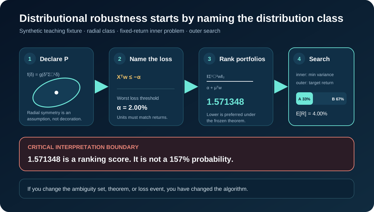
The numerator is portfolio standard deviation under Sigma. The denominator
adds the loss threshold and expected return. A lower ratio receives the lower
worst-case loss ranking under the theorem.
Here is the boundary I want visible on every screen: the ratio is called
risk_score. A score of 1.57 is not a 157% probability. The theorem gives an
equivalent minimizer under its class; it does not say the raw ratio is a
universal probability measure.
Why the solution becomes manageable
Fix beta=mu^T w. At that one expected return, the denominator is fixed, so we
only need the portfolio with minimum variance:
minimize w^T Sigma w
subject to the long-only simplex and mu^T w=beta. This is a convex quadratic
frontier problem. We solve it for candidate beta values between the feasible
floor and the maximum asset mean, evaluate the ratio, and perform a bounded
one-dimensional search.
A QP solver can certify one inner point. It cannot by itself certify that the outer search is complete. Production code should retain both levels of status.
A synthetic example with a binding floor
Use:
mu = [0.06, 0.03]
Sigma = [[0.04, 0.00],
         [0.00, 0.01]]
alpha = 0.02
gamma = 0.04
At equal weights, expected return is 0.045, variance is 0.0125, and
risk_score=sqrt(0.0125)/(0.02+0.045)=1.72005229.
Asset B alone has lower variance, but its expected return is 0.03, below the
floor. Writing w=[x,1-x], the floor requires x>=1/3. The unconstrained ratio
minimum occurs below that boundary, so the constrained optimum sits exactly at
x=1/3.
The result is:
weights = [0.3333333333, 0.6666666667]
expected return = 0.04
variance = 0.0088888889
risk_score = 1.5713484026
Every value is author-derived from synthetic moments. No observed asset or future performance is implied.
The equation-level evidence matters
An earlier research note for this topic deliberately stopped because the primary equation could not be inspected. That was the right decision. Calling an optimizer DRO while guessing its ambiguity class is a critical error.
The NIH/PMC author manuscript is now accessible and exposes the long-only set, radial density conditions, worst-loss definition, constrained problem, ratio reformulation, and theorem. That closes the mathematical blocker. It does not close the empirical question of whether this class is suitable for a specific portfolio.
Input validation cannot be delegated to DRO
The optimizer consumes mean and covariance. Those moments can still be wrong because a split was handled inconsistently, a cash dividend disappeared from wealth, a price belonged to the wrong date or instrument, or quantities from old holdings changed unit. Multi-currency portfolios add another layer: every return must share a declared reporting currency and FX timestamp.
I treat those checks as hard gates. Distributional ambiguity is not a bucket for arbitrary data corruption. If a return row is economically impossible, reject or repair it through a governed source process before estimating the moments. Do not enlarge an ambiguity set to hide a broken security master.
Implementation walkthrough
The Python reference and TypeScript reference enumerate active asset subsets for each fixed-return inner problem and then use the same golden-section search across the feasible return interval. This small- universe design is readable and deterministic.
The function rejects non-positive alpha, an infeasible gamma, indefinite
covariance, a singular solve, and a non-positive denominator. Its output carries
an interpretation string so a consumer does not silently relabel the score.
For larger universes, replace the reference solver with a mature QP and a
documented scalar-search wrapper; do not change the contract.
Use the lab as a model review
Open the distributionally robust portfolio playground.
Step through the class, loss event, feasible return interval, fixed-return
frontier, and final score. Raise gamma and watch the feasible set contract.
Raise alpha and observe the denominator change. The failure scenario puts the
floor above every asset mean and stops before any solver result appears.
The lab never simulates colorful paths and calls the picture DRO. Monte Carlo
can illustrate distributions, but here the mathematical result is defined by
the supremum over F and the theorem's equivalent optimization.
Tests and claims
Tests reproduce the equal-weight score and the binding-floor optimum, verify the return constraint, tighten the floor, reject an impossible floor, reject a zero threshold, reject indefinite covariance, and compare Python with TypeScript. The fixed fixture lets an independent reviewer solve the scalar boundary by hand.
The historical-example decision is deferred. A named market case needs a licensed point-in-time panel, complete adjustment and currency basis, and evidence that the radial class is an appropriate modeling choice. The primary paper's academic examples support the method; they are not republished here as market performance evidence.
What this result does not mean
It does not mean the future distribution lies in F. It does not calibrate the
bounded-support parameter, estimate mu or Sigma, or model costs, liquidity,
taxes, leverage, or path-dependent drawdown. It does not prove a lower score
will earn more money. And it does not let us transfer Wasserstein or moment-set
guarantees into this radial model.
Distributional robustness is valuable because the ambiguity is explicit. It becomes misleading the moment the class, loss event, or theorem boundary is hidden behind one “risk” number.
Summary
An auditable DRO portfolio begins with four visible objects: an ambiguity class, a loss event, a feasible holdings set, and a result whose interpretation matches the theorem. For the selected radial class, fixed-return variance problems plus a scalar search provide a transparent implementation. The score ranks worst-loss probability under the source conditions; it is not itself a universal probability.
Next, Kelly Allocation keeps supplied scenario probabilities fixed but changes the objective to expected logarithmic wealth.
Choose the family method by the decision you face
| Your real question | Start with | What changes | What it does not solve |
|---|---|---|---|
| How should uncertain views modify a market prior? | Black-Litterman | Expected returns through a prior and views | Distributional ambiguity |
| How unstable are optimized weights across plausible samples? | Resampled Efficient Frontier | Rows, replicate moments, and rank-matched frontiers | A worst-distribution objective |
| How should a bounded error in the mean affect allocation? | Robust Mean-Variance | Mean vector inside a declared ellipsoid | Ambiguity about the whole return law |
| Which portfolio ranks best under a declared distribution class and loss event? | Distributionally Robust Portfolio | The admissible return distribution | Universal safety or a probability label for the ratio |
| Which scenario mix maximizes long-run log growth? | Kelly Allocation | Objective and scenario wealth factors | Protection against an unspecified distribution class |
Related concepts and learning handoff
The reviewed The Fintech Builder chapter KKT checks and limits of an optimality claim (17:33–18:43) supports review of each fixed-return inner problem. It does not establish the radial-class theorem, turn the ratio into a probability, or transfer guarantees from another ambiguity set.
Rendered from the canonical Mermaid sources linked by this article.
distributionally robust flow
ReferencesPrimary sources and evidence notesExpand the source trail, evidence role, and limitations behind the engineering choices.
Expand the source trail, evidence role, and limitations behind the engineering choices.
BL2019 — Distributionally Robust Portfolio Optimization
- Organization or authors: I. E. Bardakci and C. M. Lagoa.
- Source type: Original peer-reviewed IEEE conference paper; NIH/PMC author manuscript.
- Publication or effective date: December 2019, CDC 2019, pages 1526–1531.
- Version: DOI
10.1109/CDC40024.2019.9029381; PMC7956065. - URL or DOI: NIH/PMC author manuscript, Penn State record.
- Accessed: 2026-09-15.
- Jurisdiction: None; mathematical portfolio methodology.
- Supports: Radial admissible density class, equations (2)–(5), worst-case loss probability, equivalent ratio minimization, and QP plus one-dimensional search.
- Limitations: The equivalence is conditional on the paper's class and theorem; the ratio is not an unconditional probability.
DY2010 — Distributionally Robust Optimization Under Moment Uncertainty
- Organization or authors: Alexandre Delage and Yinyu Ye.
- Source type: Original peer-reviewed Operations Research article.
- Publication or effective date: 2010, 58(3), 595–612.
- Version: DOI
10.1287/opre.1090.0741. - URL or DOI: INFORMS record.
- Accessed: 2026-09-15.
- Jurisdiction: None.
- Supports: Moment-confidence-region DRO as a major nearby formulation with a portfolio application.
- Limitations: It is not silently substituted for the radial class.
EK2018 — Data-driven DRO using the Wasserstein metric
- Organization or authors: Peyman Mohajerin Esfahani and Daniel Kuhn.
- Source type: Original peer-reviewed Mathematical Programming article and author manuscript.
- Publication or effective date: 2018, 171, 115–166.
- Version: DOI
10.1007/s10107-017-1172-1. - URL or DOI: Author manuscript.
- Accessed: 2026-09-15.
- Jurisdiction: None.
- Supports: Wasserstein-ball DRO as a distinct data-driven alternative.
- Limitations: Its guarantees and reformulations do not apply automatically to this package's radial ambiguity class.
Full dependency-light reference implementations in both supported languages.
export class ContractError extends Error{};type V=number[];type M=number[][];const dot=(a:V,b:V)=>a.reduce((s,x,i)=>s+x*b[i],0),mv=(a:M,x:V)=>a.map(r=>dot(r,x));
function solve(a:M,b:V):V{const n=b.length,g=a.map((r,i)=>[...r,b[i]]);for(let c=0;c<n;c++){let p=c;for(let r=c+1;r<n;r++)if(Math.abs(g[r][c])>Math.abs(g[p][c]))p=r;if(Math.abs(g[p][c])<=1e-14)throw new ContractError("singular system");[g[c],g[p]]=[g[p],g[c]];const z=g[c][c];g[c]=g[c].map(v=>v/z);for(let r=0;r<n;r++)if(r!==c){const f=g[r][c];g[r]=g[r].map((v,j)=>v-f*g[c][j]);}}return g.map(r=>r[n]);}
function* combos(n:number,k:number,s=0,p:number[]=[]):Generator<number[]>{if(p.length===k){yield p;return}for(let i=s;i<n;i++)yield*combos(n,k,i+1,[...p,i]);}
function spd(s:M){const n=s.length;if(s.some((r,i)=>r.some((x,j)=>Math.abs(x-s[j][i])>1e-12)))throw new ContractError("covariance must be symmetric");const l=Array.from({length:n},()=>Array(n).fill(0));for(let i=0;i<n;i++)for(let j=0;j<=i;j++){const z=s[i][j]-Array.from({length:j},(_,k)=>l[i][k]*l[j][k]).reduce((a,b)=>a+b,0);if(i===j){if(z<=1e-14)throw new ContractError("covariance must be positive definite");l[i][j]=Math.sqrt(z)}else l[i][j]=z/l[j][j]}}
function fixedTarget(mu:V,sigma:M,target:number):V{const n=mu.length;let best:{v:number,w:V}|undefined;for(let size=1;size<=n;size++)for(const active of combos(n,size)){const w=Array(n).fill(0);if(size===1){if(Math.abs(mu[active[0]]-target)>1e-9)continue;w[active[0]]=1}else{const sub=active.map(i=>active.map(j=>sigma[i][j]));let io:V,im:V;try{io=solve(sub,Array(size).fill(1));im=solve(sub,active.map(i=>mu[i]))}catch{continue}const a=io.reduce((x,y)=>x+y,0),b=active.reduce((s,x,i)=>s+mu[x]*io[i],0),c=active.reduce((s,x,i)=>s+mu[x]*im[i],0),det=a*c-b*b;if(Math.abs(det)<=1e-14)continue;const l1=(c-b*target)/det,l2=(a*target-b)/det,sw=io.map((x,i)=>l1*x+l2*im[i]);if(Math.min(...sw)<=1e-11)continue;active.forEach((x,i)=>w[x]=sw[i])}const v=dot(w,mv(sigma,w));if(!best||v<best.v-1e-14)best={v,w}}if(!best)throw new ContractError("fixed-return frontier is infeasible");return best.w;}
function gmv(mu:V,sigma:M):V{const n=mu.length;let best:{v:number,w:V}|undefined;for(let size=1;size<=n;size++)for(const active of combos(n,size)){let w=Array(n).fill(0);if(size===1)w[active[0]]=1;else{const sub=active.map(i=>active.map(j=>sigma[i][j]));let io:V;try{io=solve(sub,Array(size).fill(1))}catch{continue}const sw=io.map(x=>x/io.reduce((a,b)=>a+b,0));if(Math.min(...sw)<=1e-11)continue;active.forEach((x,i)=>w[x]=sw[i])}const v=dot(w,mv(sigma,w));if(!best||v<best.v-1e-14)best={v,w}}if(!best)throw new ContractError("simplex infeasible");return best.w;}
export interface DroResult{weights:V;expectedReturn:number;variance:number;riskScore:number;lossThreshold:number;returnFloor:number;outerIterations:number;status:"optimal";interpretation:string}
export function distributionallyRobustPortfolio(mean:V,covariance:M,lossThreshold:number,returnFloor:number,tolerance=1e-11,maxIterations=160):DroResult{const mu=mean.map(Number),n=mu.length,sigma=covariance.map(r=>r.map(Number));if(!n||mu.some(x=>!Number.isFinite(x)))throw new ContractError("mean must be finite");if(sigma.length!==n||sigma.some(r=>r.length!==n)||sigma.flat().some(x=>!Number.isFinite(x)))throw new ContractError("covariance shape/values invalid");spd(sigma);if(!(lossThreshold>0))throw new ContractError("lossThreshold alpha must be positive");if(!Number.isFinite(returnFloor)||returnFloor>Math.max(...mu)+1e-12)throw new ContractError("return floor is infeasible");const lo=Math.max(returnFloor,Math.min(...mu)),hi=Math.max(...mu);if(lossThreshold+lo<=0)throw new ContractError("alpha + feasible expected return must be positive");if(!(tolerance>0)||maxIterations<1)throw new ContractError("outer search controls invalid");const evaluate=(beta:number)=>{const w=hi-lo>1e-13?fixedTarget(mu,sigma,beta):gmv(mu,sigma),variance=dot(w,mv(sigma,w));return{score:Math.sqrt(Math.max(variance,0))/(lossThreshold+dot(mu,w)),w,variance}};let winner,iterations=0;if(hi-lo<=tolerance)winner=evaluate(lo);else{const gr=(Math.sqrt(5)-1)/2;let a=lo,b=hi,c=b-gr*(b-a),d=a+gr*(b-a),fc=evaluate(c),fd=evaluate(d);while(b-a>tolerance&&iterations<maxIterations){if(fc.score<=fd.score){b=d;d=c;fd=fc;c=b-gr*(b-a);fc=evaluate(c)}else{a=c;c=d;fc=fd;d=a+gr*(b-a);fd=evaluate(d)}iterations++}winner=[evaluate(lo),evaluate(hi),fc,fd].sort((x,y)=>x.score-y.score)[0]}return{weights:winner.w,expectedReturn:dot(mu,winner.w),variance:winner.variance,riskScore:winner.score,lossThreshold,returnFloor,outerIterations:iterations,status:"optimal",interpretation:"riskScore ranks worst-case loss probability only under the cited radial-class theorem; it is not itself an unconditional probability"};}
The embedded lab now expands to its full document height, keeping the article as the only scroll surface.