
 By Islam Baraka
For analysts and developers who know decimal log returns, sample variance, and consistently adjusted OHLC bars. The goal is to reproduce the mechanism, inspect its failure states, and decide what the output can legitimately tell you—not to fit or endorse a trading strategy.
A stock can finish exactly where it started after a very uncomfortable day. Close-to-close volatility will not describe that journey. It answers a narrower, useful question: how dispersed were the returns between successive closes?
That narrowness is a strength when you are building a risk pipeline. You can trace every number back to two prices, explain the denominator, and reproduce the result without an intraday feed. Start with that auditable baseline. Add a more elaborate estimator only when you can explain what extra information it contributes.
By the end, you should be able to compute the estimate, identify its first valid observation, and explain why a large overnight move and a large intraday excursion are not interchangeable inputs. You need logarithms, a mean, and sample variance—not a forecasting model.
Open this figure at full size.
What exactly is being estimated?
Let C_t be a consistently adjusted session close. The decimal log return is r_t = ln(C_t/C_(t-1)). A 1% simple return corresponds to ln(1.01), approximately 0.00995033; do not enter the number 1 for 1%.
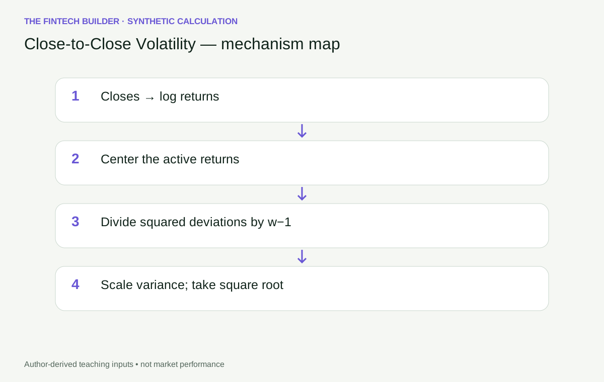
For w returns, subtract their sample mean, square each deviation, add the squares, and divide by w−1. Multiply the resulting variance by an explicitly chosen annualization factor A. Volatility is the square root of that annualized variance. The TTR technical reference documents this close-based convention alongside the range estimators.
The denominator and centering are not interchangeable settings. Mean squared returns, sample variance, and maximum-likelihood variance are different quantities. If all observed log returns equal 0.01, their sample variance is zero even though the price rises every session. The estimator measures dispersion around the sample mean, not the total distance travelled by the price.
A calculation small enough to check by hand
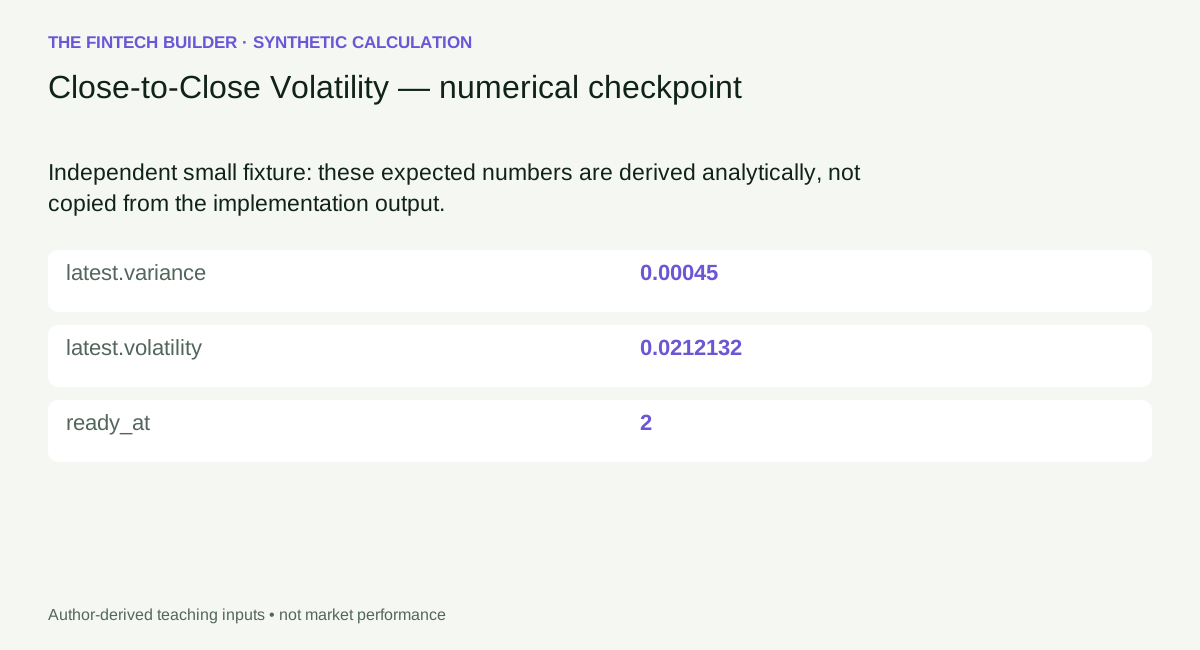
Take three synthetic closes with log-price offsets 0, 0.01 and −0.01 relative to a base price of 100. Their prices are 100, 100e^0.01 and 100e^−0.01. The two close returns are therefore +0.01 and −0.02.
Their mean is −0.005. The deviations are +0.015 and −0.015. The sum of squared deviations is 0.00045. With w=2, the divisor is one, so the unannualized sample variance is 0.00045 and volatility is approximately 0.0212132, or 2.12132% per session under the session-return interpretation.
With A=252, the variance becomes 0.1134 and the displayed annualized volatility is about 33.67%. That multiplication assumes the session variance is representative and scales linearly over the chosen horizon. It is a convention, not evidence that the next year's volatility will equal that number.
Open this figure at full size.
Download the exact worked input and expected values.
The one-row error that changes the whole chart
Two returns require three closes. More generally, a w-return window requires w+1 prices. The first price establishes a starting point; it is not a zero return.
The implementation leaves the output unavailable until it has the complete history. It never invents a previous close, inserts zero, or shortens the first window. For w=12, the first valid output is at zero-based index 12. Every subsequent output uses the last 12 returns and therefore 13 closes.
When streaming data, calculate only after the final close used by the window is available. A revised close or corporate-action adjustment can legitimately change historical estimates. Store the data snapshot and adjustment basis if a historical decision must remain reproducible.
What a disagreement with another estimator tells you
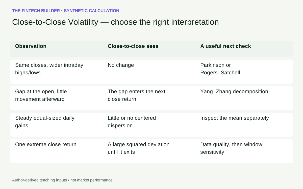
| Observation | Close-to-close sees | A useful next check |
|---|---|---|
| Same closes, wider intraday highs/lows | No change | Parkinson or Rogers–Satchell |
| Gap at the open, little movement afterward | The gap enters the next close return | Yang–Zhang decomposition |
| Steady equal-sized daily gains | Little or no centered dispersion | Inspect the mean separately |
| One extreme close return | A large squared deviation until it exits | Data quality, then window sensitivity |
A disagreement is not automatically a bug. First align sessions, price adjustments, window length, centering and annualization. Comparing annualized close volatility with unannualized realized variance compares different units as well as different estimators.
Open this figure at full size.
Use the playground as a rolling-window debugger
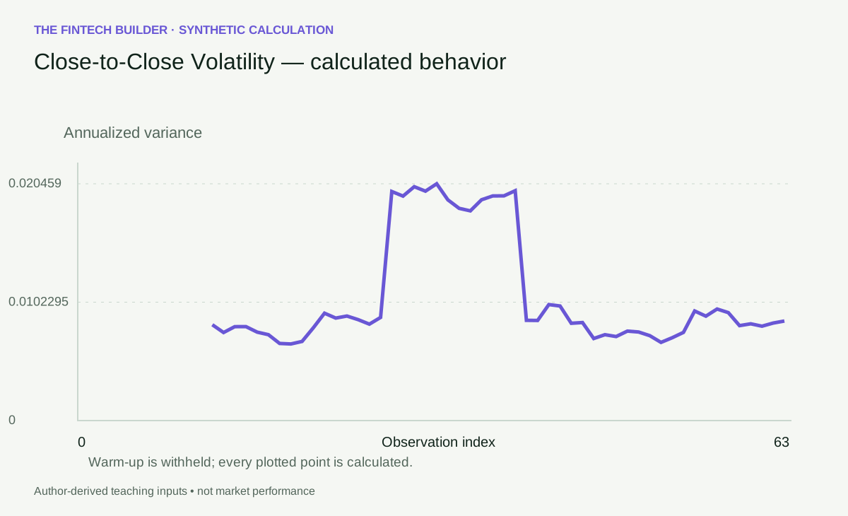
The synthetic path contains 64 observations, including a conspicuous move. Step adds one observed bar; Back removes it. The chart and contribution table are recalculated from the visible prefix. Change the return window and watch both the readiness boundary and the set of included observations change.
Predict what will happen before stepping past the large move's exit: the output can drop even if the newest return is ordinary. That is a window-membership effect, not a sudden discovery about today's market. Then inspect the flat-path edge case and malformed-bar rejection. Zero dispersion is a valid measurement; invalid input is not.
Open this figure at full size.
Open the standalone guided playground. The embedded playground and runnable code are available on this page. Download the 64-observation teaching input.
Implementation choices worth keeping
The reference performs direct window calculations because each intermediate is easy to inspect. It has O(nw) time for n observations and window w. A production stream may use a stable rolling-variance algorithm, but should retain these fixtures as an independent behavioral check. Naively subtracting two large nearly equal accumulated sums can lose precision.
Prices must be positive and finite. UTC timestamps must be real calendar dates and strictly increasing. The teaching OHLC schema also checks high/low bracketing; only closes enter this estimator. Missing sessions are not automatically zero-return sessions. The code does not infer an exchange calendar or decide whether a closure, outage or omitted record explains a gap.
A split adjustment applied only to the final close can manufacture an enormous return. Conversely, dropping a genuine large move because it looks inconvenient understates the sample's dispersion. Resolve the data event before deciding whether to retain, correct or exclude it.
My practical reading rule
Keep three things beside the headline number: the return window, its largest squared deviations, and the annualization convention. Those explain more than an extra decimal place. Use this estimate as a transparent historical baseline—not a probability of loss, a direction signal, or a promise of future risk.
Next, compare Parkinson volatility on the same bars, then use Yang–Zhang when opening gaps matter.
Reproduce and inspect the calculation
The Python and TypeScript tabs contain standalone implementations, not imports into an unseen runtime. Both expose calculate(input_data). Feed the worked JSON's input object into that entry point. For the longer experiment, use the teaching-path JSON directly.
import json
from pathlib import Path
from close_to_close_volatility import calculate

data = json.loads(Path("teaching-path.json").read_text())
result = calculate(data)
print(result["latest"])
import {calculate} from './close_to_close_volatility.ts';
const result = calculate(inputData); // inputData is the downloaded JSON object
console.log(result.latest);
Place the downloaded input beside your script and the standalone source on its import path. The Python reference uses the standard library; the TypeScript reference has no external runtime dependency. Shared tests include independent numeric anchors, valid boundaries, rejected inputs and cross-language output comparisons. They establish arithmetic, not forecasting performance.
Evidence and scope
This article uses authored synthetic calculations and primary technical references, reviewed 2026-09-10. Historical market examples are deferred until identity, adjustment basis, chronology and redistribution rights can be verified. No personal trading history or search-ranking superiority is asserted.
w returns require w+1 closes; sample centering; no inferred exchange calendar.
Continue the investigation
- Parkinson Volatility: compare its assumptions and information boundary before comparing the numbers.
- Yang-Zhang Volatility: compare its assumptions and information boundary before comparing the numbers.
Rendered from the canonical Mermaid sources linked by this article.
Close-to-Close Volatility — calculation-flow
Close-to-Close Volatility — decision-boundary
ReferencesPrimary sources and evidence notesExpand the source trail, evidence role, and limitations behind the engineering choices.
Expand the source trail, evidence role, and limitations behind the engineering choices.
Reviewed 2026-09-10. Primary technical documentation and papers; synthetic arithmetic is author-derived. This is a targeted source review, not a verified review of Google's top ten results and not a claim of ranking superiority.
- S1: TTR — volatility: close and range estimator conventions — accessed 2026-09-10. Rolling official documentation snapshot; exact package versions used for numerical comparisons are recorded in the repair numeric-evidence.json. Supports the definition and declared convention, not investment performance. Jurisdiction: not applicable to this mathematical reference.
Scope of evidence
w returns require w+1 closes; sample centering; no inferred exchange calendar.
Historical case: deferred. No public provider dataset, historical performance claim, or personal trading anecdote is used. Synthetic examples demonstrate arithmetic, not market efficacy. Sources are not copied as article prose.
Accessed: 2026-09-10.
Supports: estimator definition and the explicitly declared variants.
Limitations: technical documentation does not verify a real market feed, author experience, forecast efficacy or search-result superiority. Original-paper access limitations are recorded in the repair report.
Full dependency-light reference implementations in both supported languages.
/** Standalone D10-F01-A01 reference. Generated from validated D10 v2 source. */
export class ContractError extends Error {}
type RecordValue=Record<string, any>;
type Matrix=number[][];
const sum=(x:number[]):number=>x.reduce((a,b)=>a+b,0);


function requireValue(ok: unknown, code: string, message: string): asserts ok {
  if (!ok) throw new ContractError(`${code}: ${message}`);
}

function finite(x: unknown, name: string): number {
  requireValue(typeof x === 'number' && Number.isFinite(x), 'NUMBER', `${name} must be a finite number`);
  return x;
}

function integer(x: unknown, name: string, minimum = 0, maximum = 10000): number {
  const v = finite(x, name);
  requireValue(Number.isInteger(v) && v >= minimum && v <= maximum, 'INTEGER', `${name} must be an integer in [${minimum}, ${maximum}]`);
  return v;
}

function param(p: RecordValue, key: string, fallback: number): number {
  return finite(Object.hasOwn(p, key) ? p[key] : fallback, key);
}

function option(p: RecordValue, key: string, fallback: any): any {
  return Object.hasOwn(p, key) ? p[key] : fallback;
}

function positive(p: RecordValue, key: string, fallback: number): number {
  const v = param(p, key, fallback);
  requireValue(v > 0, 'RANGE', `${key} must be positive`);
  return v;
}

function timestamps(values: unknown, n: number, name: string, regular = false): number[] {
  requireValue(Array.isArray(values) && values.length === n, 'TIME', `${name} must match observation count`);
  const result: number[] = [];
  for (const value of values) {
    requireValue(typeof value === 'string' && /^\d{4}-\d{2}-\d{2}T\d{2}:\d{2}:\d{2}(?:\.\d{3})?Z$/.test(value), 'TIME', 'use UTC ISO timestamps');
    const instant = Date.parse(value);
    const canonical = value.length === 20 ? value.replace('Z', '.000Z') : value;
    requireValue(Number.isFinite(instant) && Number(value.slice(0, 4)) >= 1000 && new Date(instant).toISOString() === canonical, 'TIME', 'invalid calendar timestamp');
    requireValue(!result.length || instant > result[result.length - 1], 'TIME', 'timestamps must strictly increase');
    result.push(instant);
  }
  if (regular && n > 2) requireValue(result.slice(2).every((v, i) => v - result[i + 1] === result[1] - result[0]), 'ALIGNMENT', 'returns need a regular grid');
  return result;
}

function bars(data: RecordValue): any[][] {
  const values = data.bars;
  requireValue(Array.isArray(values) && values.length >= 2 && values.every(b => b && typeof b === 'object' && !Array.isArray(b)), 'SHAPE', 'bars needs at least two OHLC objects');
  timestamps(values.map(b => b.timestamp), values.length, 'bars.timestamp');
  return values.map(b => {
    const [o, h, l, c] = ['open', 'high', 'low', 'close'].map(k => finite(b[k], k));
    requireValue(Math.min(o, h, l, c) > 0 && h >= Math.max(o, c) && l <= Math.min(o, c), 'OHLC', 'positive bracketed OHLC required');
    return [b.timestamp, o, h, l, c];
  });
}

function variance(x: number[]): number {
  const mean = sum(x) / x.length;
  return sum(x.map(v => (v - mean) ** 2)) / (x.length - 1);
}

function seriesResult(series: (RecordValue | null)[], diagnostics: RecordValue): RecordValue {
  const at = series.findIndex(v => v !== null);
  return {series, latest: series.at(-1) ?? null, ready: series.length > 0 && series.at(-1) !== null,
    ready_at: at < 0 ? null : at, diagnostics};
}

function historical(data: RecordValue, p: RecordValue, kind: string): RecordValue {
  const values = bars(data), w = integer(option(p, 'window', 12), 'window', 2), scale = positive(p, 'annualization_factor', 252);
  const contributions = values.map(([, o, h, l, c], i) => {
    const rs = Math.log(h / c) * Math.log(h / o) + Math.log(l / c) * Math.log(l / o);
    const choices: RecordValue = {
      close_to_close: i === 0 ? null : Math.log(c / values[i - 1][4]),
      parkinson: Math.log(h / l) ** 2 / (4 * Math.log(2)),
      garman_klass: .5 * Math.log(h / l) ** 2 - (2 * Math.log(2) - 1) * Math.log(c / o) ** 2,
      rogers_satchell: rs,
      yang_zhang: [i === 0 ? null : Math.log(o / values[i - 1][4]), Math.log(c / o), rs],
    };
    return choices[kind];
  });
  const series = values.map((bar, i) => {
    const block = contributions.slice(Math.max(0, i - w + 1), i + 1);
    if (block.length < w || block.some(v => v === null) || (kind === 'yang_zhang' && block[0][0] === null)) return null;
    let estimate: number, components: RecordValue = {};
    if (kind === 'yang_zhang') {
      const overnight = variance(block.map(v => v[0])), intraday = variance(block.map(v => v[1]));
      const rs = sum(block.map(v => v[2])) / w, k = .34 / (1.34 + (w + 1) / (w - 1));
      estimate = scale * (overnight + k * intraday + (1 - k) * rs);
      components = {overnight: scale * overnight, open_close: scale * k * intraday, range: scale * (1 - k) * rs, k};
    } else estimate = scale * (kind === 'close_to_close' ? variance(block) : sum(block) / w);
    requireValue(estimate >= 0, 'NUMERIC', 'negative variance: inspect inputs and precision');
    return {timestamp: bar[0], variance: estimate, volatility: Math.sqrt(estimate), contributions: block, components, window_start: i - w + 1, window_end: i};
  });
  return seriesResult(series, {input_count: values.length, annualization_factor: scale, causal: true});
}
export function calculate(data: RecordValue): RecordValue {
  requireValue(data && typeof data === 'object' && !Array.isArray(data),'SHAPE','input must be an object');
  const p=Object.hasOwn(data,'parameters')?data.parameters:{};
  requireValue(p && typeof p === 'object' && !Array.isArray(p),'SHAPE','parameters must be an object');
  const result=historical(data,p,"close_to_close");
  function check(v:any):void {
    if(typeof v==='number')requireValue(Number.isFinite(v),'NUMERIC','nonfinite computed output');
    else if(Array.isArray(v))v.forEach(check);
    else if(v && typeof v==='object')Object.values(v).forEach(check);
  }
  check(result);
  return {topic_id:"D10-F01-A01",title:"Close-to-Close Volatility",parameters:p,...result};
}
The embedded lab now expands to its full document height, keeping the article as the only scroll surface.