
 By Islam Baraka
For analysts and developers who know decimal interval returns, regular sampling grids, and variance versus volatility. The goal is to reproduce the mechanism, inspect its failure states, and decide what the output can legitimately tell you—not to fit or endorse a trading strategy.
Two intraday paths can have the same final return and very different accumulated variation. Realized variance makes that difference measurable: square each sampled log return and add the squares.
The arithmetic is easy. The hard part is deciding what the observations represent. Sampling frequency, session boundaries and price noise can matter more than the final decimal places. This tutorial connects that data decision to a calculation you can inspect one return at a time.
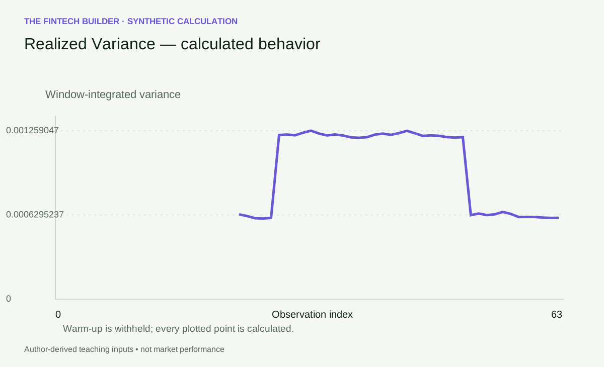
Open this figure at full size.
A sum, not the sample variance of a list
For n intraday log returns r_i covering one declared period, RV=Σr_i². There is no subtraction of the mean and no division by n or n−1. You are aggregating variation across the period, not estimating the dispersion of a randomly selected intraday return.
The theoretical connection is to quadratic variation. Under suitable sampling and price-process assumptions, increasingly fine observations reveal integrated continuous variance plus squared jumps. Market-microstructure noise changes that argument; it does not disappear just because the sampling interval becomes shorter. The realized-kernel documentation and cited research explain why lag-sensitive alternatives are used when observation noise matters.
The package defaults to A=1, so its output is variance integrated over the chosen window. An optional positive multiplier A rescales it. Calling that multiplier 252 is appropriate only when the window represents the daily quantity you intend to annualize. A 24-return window is not automatically a trading day.
Four returns that expose the mechanism
Take synthetic decimal returns [0.01,−0.02,0.03,−0.01]. Their squares are [0.0001,0.0004,0.0009,0.0001]. Add them to obtain RV=0.0015. Realized volatility is √0.0015≈0.0387298, or 3.87298% over this four-interval window.
The net log return is only 0.01. Squaring that net return gives 0.0001, not 0.0015. The difference is exactly why the path matters. Netting positive and negative returns before squaring throws away movement that RV is designed to retain.
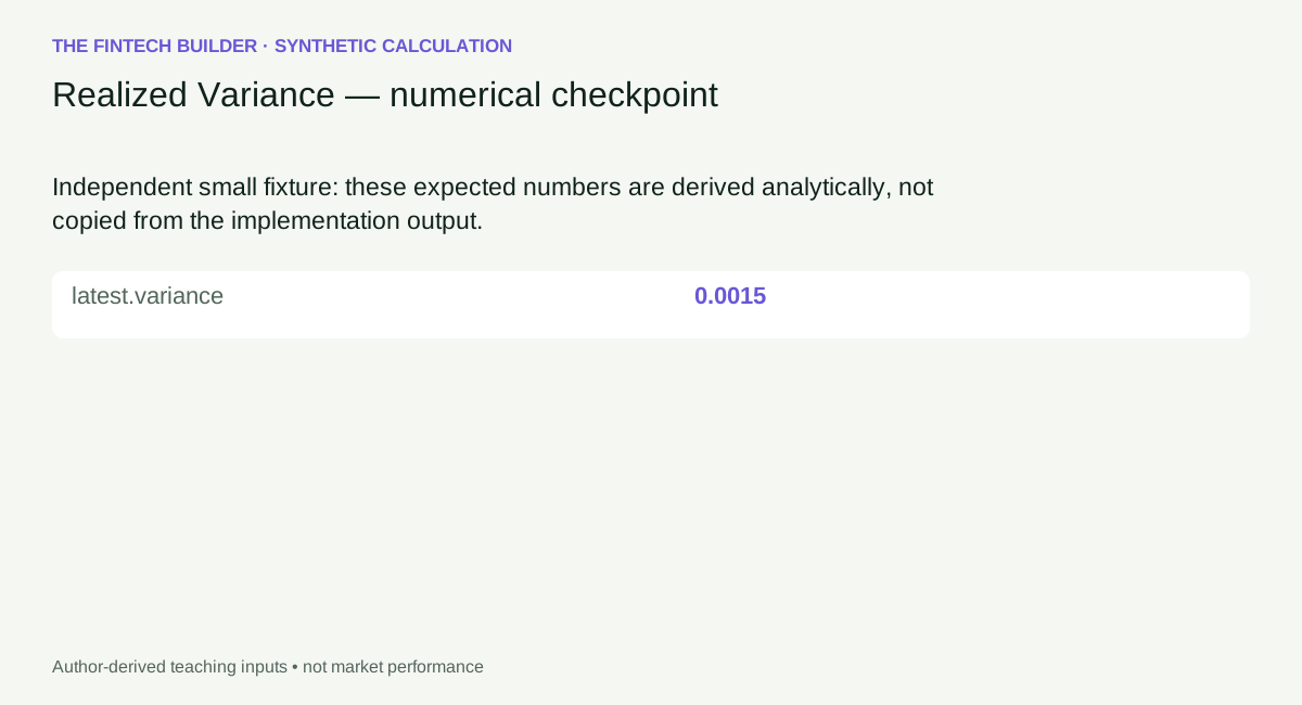
Open this figure at full size.
Download the exact worked input and expected values.
Resampling changes cross terms
Combine the first two intervals and the last two. The aggregated log returns are−0.01 and 0.02, giving RV=0.0005. This is not an implementation contradiction. Algebra says (a+b)²=a²+b²+2ab. When adjacent returns have opposite signs, their cross term is negative and coarser sampling can reduce the sum of squares.
Now imagine a constant latent price observed with an alternating quote error. The observed returns can bounce between positive and negative values while the underlying efficient price barely moves. Squaring those returns converts measurement noise into a positive contribution. Adding more such observations can increase RV without adding economic variation.
This thought experiment is the reason to inspect a volatility-signature plot: calculate RV at several sampling intervals while keeping the period and price construction comparable. A rising fine-grid estimate may reveal noise sensitivity. It does not, by itself, identify the uniquely correct sampling frequency.
The clock is part of the data contract
| Input choice | What must remain explicit |
|---|---|
| Trade price, midpoint or another price | Which observed process supplies returns |
| Sampling interval | The regular grid and aggregation rule |
| Session boundary | Whether opening/overnight movement is included |
| Missing observation | Reject, resample or documented upstream treatment |
| Output scale | Window-integrated variance versus annualized variance |
The runtime accepts finite decimal returns and optionally validates a regular UTC timestamp grid. If timestamps are omitted, regular-grid semantics are a caller obligation, not a fact verified by array length. It never inserts zero for a missing return. A stale price can generate zero returns followed by a delayed move; that is a data interpretation issue worth surfacing.
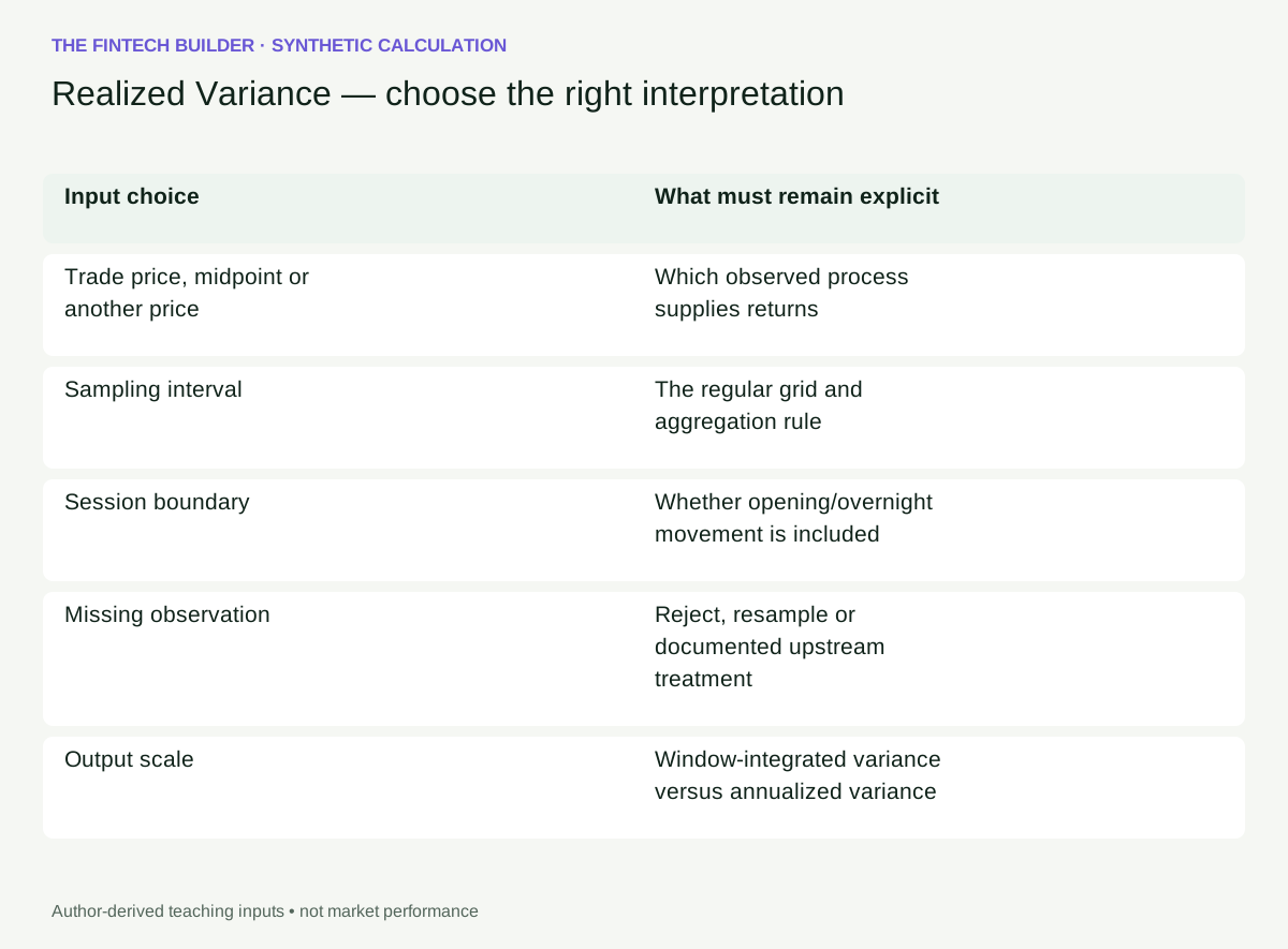
Open this figure at full size.
Step through the sum, then challenge it
The playground starts with a useful computed prefix of 64 synthetic observations. Step advances one observation and updates the rolling sum, contribution table and chart. Increase the window and predict which squared returns enter. The shock experiment makes a single term dominate; the flat-path edge case correctly produces zero.
Use the resampling discussion above as a second exercise: aggregate adjacent log returns yourself and compare their squares with the original sum. The difference should match twice the sum of adjacent cross products. A chart alone cannot teach that identity; the displayed numbers let you verify it.
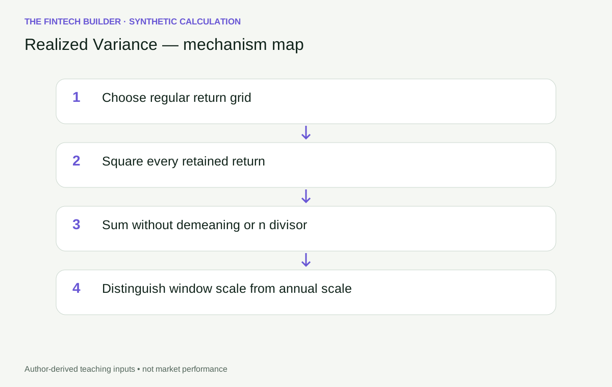
Open this figure at full size.
Open the standalone guided playground. The embedded playground and runnable code are available on this page. Download the 64-observation teaching input.
What to build around this calculation
For n observations and a rolling window w, the direct reference costs O(nw). A streaming version can maintain the sum of the latest w squared returns with an entering and leaving term. Test the warm-up boundary, every window exit, sign invariance, and scale behavior before replacing the transparent reference.
Flipping every return's sign leaves RV unchanged. Multiplying returns by c multiplies RV by c². A zero path has zero variance, whereas a null observation is invalid. These invariants catch errors that a single expected total cannot.
The result is an ex-post measurement, not a next-period forecast. It includes jump variation rather than separating it. Compare bipower variation when that distinction matters, and the finite Bartlett kernel to study how lag products change a noise-sensitive estimate.
My final question before using an RV number is: “Variation of which observed price, over which period, at which grid?” If those three answers are missing, the formula may be correct while the measurement remains ambiguous.
Reproduce and inspect the calculation
The Python and TypeScript tabs contain standalone implementations, not imports into an unseen runtime. Both expose calculate(input_data). Feed the worked JSON's input object into that entry point. For the longer experiment, use the teaching-path JSON directly.
import json
from pathlib import Path
from realized_variance import calculate

data = json.loads(Path("teaching-path.json").read_text())
result = calculate(data)
print(result["latest"])
import {calculate} from './realized_variance.ts';
const result = calculate(inputData); // inputData is the downloaded JSON object
console.log(result.latest);
Place the downloaded input beside your script and the standalone source on its import path. The Python reference uses the standard library; the TypeScript reference has no external runtime dependency. Shared tests include independent numeric anchors, valid boundaries, rejected inputs and cross-language output comparisons. They establish arithmetic, not forecasting performance.
Evidence and scope
This article uses authored synthetic calculations and primary technical references, reviewed 2026-09-10. Historical market examples are deferred until identity, adjustment basis, chronology and redistribution rights can be verified. No personal trading history or search-ranking superiority is asserted.
Decimal log returns on a declared regular grid. Default A=1 means window-integrated variance, not a per-observation average.
Continue the investigation
- Realized Covariance: compare its assumptions and information boundary before comparing the numbers.
- Realized Kernel: compare its assumptions and information boundary before comparing the numbers.
Rendered from the canonical Mermaid sources linked by this article.
Realized Variance — calculation-flow
Realized Variance — decision-boundary
ReferencesPrimary sources and evidence notesExpand the source trail, evidence role, and limitations behind the engineering choices.
Expand the source trail, evidence role, and limitations behind the engineering choices.
Reviewed 2026-09-10. Primary technical documentation and papers; synthetic arithmetic is author-derived. This is a targeted source review, not a verified review of Google's top ten results and not a claim of ranking superiority.
- S1: highfrequency — ICov estimator documentation — accessed 2026-09-10. Rolling official documentation snapshot; exact package versions used for numerical comparisons are recorded in the repair numeric-evidence.json. Supports the definition and declared convention, not investment performance. Jurisdiction: not applicable to this mathematical reference.
- S2: highfrequency — rKernelCov estimator documentation — accessed 2026-09-10. Rolling official documentation snapshot; exact package versions used for numerical comparisons are recorded in the repair numeric-evidence.json. Supports the definition and declared convention, not investment performance. Jurisdiction: not applicable to this mathematical reference.
Scope of evidence
Decimal log returns on a declared regular grid. Default A=1 means window-integrated variance, not a per-observation average.
Historical case: deferred. No public provider dataset, historical performance claim, or personal trading anecdote is used. Synthetic examples demonstrate arithmetic, not market efficacy. Sources are not copied as article prose.
Accessed: 2026-09-10.
Supports: estimator definition and the explicitly declared variants.
Limitations: technical documentation does not verify a real market feed, author experience, forecast efficacy or search-result superiority. Original-paper access limitations are recorded in the repair report.
Full dependency-light reference implementations in both supported languages.
/** Standalone D10-F02-A01 reference. Generated from validated D10 v2 source. */
export class ContractError extends Error {}
type RecordValue=Record<string, any>;
type Matrix=number[][];
const sum=(x:number[]):number=>x.reduce((a,b)=>a+b,0);


function requireValue(ok: unknown, code: string, message: string): asserts ok {
  if (!ok) throw new ContractError(`${code}: ${message}`);
}

function finite(x: unknown, name: string): number {
  requireValue(typeof x === 'number' && Number.isFinite(x), 'NUMBER', `${name} must be a finite number`);
  return x;
}

function integer(x: unknown, name: string, minimum = 0, maximum = 10000): number {
  const v = finite(x, name);
  requireValue(Number.isInteger(v) && v >= minimum && v <= maximum, 'INTEGER', `${name} must be an integer in [${minimum}, ${maximum}]`);
  return v;
}

function param(p: RecordValue, key: string, fallback: number): number {
  return finite(Object.hasOwn(p, key) ? p[key] : fallback, key);
}

function option(p: RecordValue, key: string, fallback: any): any {
  return Object.hasOwn(p, key) ? p[key] : fallback;
}

function positive(p: RecordValue, key: string, fallback: number): number {
  const v = param(p, key, fallback);
  requireValue(v > 0, 'RANGE', `${key} must be positive`);
  return v;
}

function vector(value: unknown, name: string, minimum = 1): number[] {
  requireValue(Array.isArray(value) && value.length >= minimum, 'SHAPE', `${name} needs ${minimum} or more values`);
  return value.map((v, i) => finite(v, `${name}[${i}]`));
}

function timestamps(values: unknown, n: number, name: string, regular = false): number[] {
  requireValue(Array.isArray(values) && values.length === n, 'TIME', `${name} must match observation count`);
  const result: number[] = [];
  for (const value of values) {
    requireValue(typeof value === 'string' && /^\d{4}-\d{2}-\d{2}T\d{2}:\d{2}:\d{2}(?:\.\d{3})?Z$/.test(value), 'TIME', 'use UTC ISO timestamps');
    const instant = Date.parse(value);
    const canonical = value.length === 20 ? value.replace('Z', '.000Z') : value;
    requireValue(Number.isFinite(instant) && Number(value.slice(0, 4)) >= 1000 && new Date(instant).toISOString() === canonical, 'TIME', 'invalid calendar timestamp');
    requireValue(!result.length || instant > result[result.length - 1], 'TIME', 'timestamps must strictly increase');
    result.push(instant);
  }
  if (regular && n > 2) requireValue(result.slice(2).every((v, i) => v - result[i + 1] === result[1] - result[0]), 'ALIGNMENT', 'returns need a regular grid');
  return result;
}

function seriesResult(series: (RecordValue | null)[], diagnostics: RecordValue): RecordValue {
  const at = series.findIndex(v => v !== null);
  return {series, latest: series.at(-1) ?? null, ready: series.length > 0 && series.at(-1) !== null,
    ready_at: at < 0 ? null : at, diagnostics};
}

function normalQuantile(probability: number): number {
  const a = [-39.69683028665376, 220.9460984245205, -275.9285104469687, 138.3577518672690, -30.66479806614716, 2.506628277459239];
  const b = [-54.47609879822406, 161.5858368580409, -155.6989798598866, 66.80131188771972, -13.28068155288572];
  const c = [-.007784894002430293, -.3223964580411365, -2.400758277161838, -2.549732539343734, 4.374664141464968, 2.938163982698783];
  const d = [.007784695709041462, .3224671290700398, 2.445134137142996, 3.754408661907416];
  const poly = (co: number[], x: number) => co.slice(1).reduce((v, coefficient) => v * x + coefficient, co[0]);
  if (probability < .02425 || probability > .97575) {
    const q = Math.sqrt(-2 * Math.log(Math.min(probability, 1 - probability)));
    const value = poly(c, q) / (poly(d, q) * q + 1);
    return probability < .5 ? value : -value;
  }
  const q = probability - .5;
  return poly(a, q * q) * q / (poly(b, q * q) * q * q + 1);
}

function realized(data: RecordValue, p: RecordValue, kind: string): RecordValue {
  const key = kind === 'realized_covariance' ? 'returns_x' : 'returns', r = vector(data[key], key);
  const w = integer(option(p, 'window', 24), 'window', kind === 'jump_detector' ? 3 : 2), scale = positive(p, 'annualization_factor', 1);
  let y: number[] = [];
  if (kind === 'realized_covariance') {
    y = vector(data.returns_y, 'returns_y');
    const tx = timestamps(data.timestamps_x, r.length, 'timestamps_x', true), ty = timestamps(data.timestamps_y, y.length, 'timestamps_y', true);
    requireValue(tx.length === ty.length && tx.every((v, i) => v === ty[i]), 'ALIGNMENT', 'x/y intervals must match exactly');
  } else if (Object.hasOwn(data, 'timestamps')) timestamps(data.timestamps, r.length, 'timestamps', true);
  const alpha = kind === 'jump_detector' ? param(p, 'alpha', .05) : null;
  if (alpha !== null) requireValue(alpha >= 1e-6 && alpha < .5, 'RANGE', 'alpha must be in [0.000001, 0.5)');
  const bandwidth = kind === 'realized_kernel' ? integer(option(p, 'bandwidth', Math.min(4, w - 1)), 'bandwidth', 0, w - 1) : 0;
  const series = r.map((_, i) => {
    if (i + 1 < w) return null;
    const x = r.slice(i - w + 1, i + 1), squares = x.map(v => v * v), rv = scale * sum(squares);
    const products = x.slice(1).map((v, j) => Math.abs(v * x[j])), bv = scale * Math.PI / 2 * sum(products);
    let item: RecordValue;
    if (kind === 'realized_variance') item = {variance: rv, volatility: Math.sqrt(rv), contributions: squares.map(v => scale * v)};
    else if (kind === 'realized_covariance') {
      const paired = x.map((v, j) => scale * v * y[i - w + 1 + j]);
      item = {covariance: sum(paired), contributions: paired};
    } else if (kind === 'bipower_variation') item = {realized_variance: rv, bipower_variation: bv, signed_difference: rv - bv, jump_variation: Math.max(rv - bv, 0), contributions: products.map(v => scale * Math.PI / 2 * v)};
    else if (kind === 'jump_detector') {
      const mu43 = .8308609250295592;
      const tq = scale ** 2 * w * w / (w - 2) * sum(x.slice(2).map((v, j) => Math.abs(v * x[j + 1] * x[j]) ** (4 / 3))) / mu43 ** 3;
      const se = Math.sqrt((Math.PI ** 2 / 4 + Math.PI - 5) * tq / w), z = se > 0 ? (rv - bv) / se : null;
      const q = normalQuantile(1 - alpha!);
      item = {realized_variance: rv, bipower_variation: bv, tripower_quarticity: tq, standard_error: se, statistic: z,
        critical_value: q, jump_detected: z === null ? null : z > q, decision_status: z === null ? 'withheld-zero-quarticity' : 'asymptotic', signed_difference: rv - bv};
    } else {
      const lags = Array.from({length: bandwidth + 1}, (_, h) => {
        const gamma = sum(x.slice(h).map((v, j) => v * x[j])), weight = 1 - h / (bandwidth + 1);
        return {lag: h, weight, gamma, contribution: scale * (h === 0 ? 1 : 2) * weight * gamma};
      });
      const value = sum(lags.map(v => v.contribution));
      requireValue(value >= -1e-12 * Math.max(rv, 1e-300), 'NUMERIC', 'Bartlett quadratic form became negative');
      item = {realized_kernel: Math.max(value, 0), volatility: Math.sqrt(Math.max(value, 0)), bandwidth, lags};
    }
    return {...item, window_start: i - w + 1, window_end: i};
  });
  return seriesResult(series, {causal: true, input_count: r.length, annualization_factor: scale});
}
export function calculate(data: RecordValue): RecordValue {
  requireValue(data && typeof data === 'object' && !Array.isArray(data),'SHAPE','input must be an object');
  const p=Object.hasOwn(data,'parameters')?data.parameters:{};
  requireValue(p && typeof p === 'object' && !Array.isArray(p),'SHAPE','parameters must be an object');
  const result=realized(data,p,"realized_variance");
  function check(v:any):void {
    if(typeof v==='number')requireValue(Number.isFinite(v),'NUMERIC','nonfinite computed output');
    else if(Array.isArray(v))v.forEach(check);
    else if(v && typeof v==='object')Object.values(v).forEach(check);
  }
  check(result);
  return {topic_id:"D10-F02-A01",title:"Realized Variance",parameters:p,...result};
}
The embedded lab now expands to its full document height, keeping the article as the only scroll surface.