
 By Islam Baraka
The governed definitions this build depends on. Read them first if a term is unfamiliar.
- PrimarySector Diffusion IndexSector Diffusion Index summarizes how broadly a declared condition is spreading across eligible sectors.
- PrerequisiteDiffusion IndexDiffusion Index summarizes the balance of increases, unchanged observations, and decreases across a population.
- PrerequisiteMarket BreadthMarket breadth describes how widely a market movement is shared across its eligible securities.
- PrerequisiteSector ClassificationSector Classification is a governed taxonomy and point-in-time mapping that assigns securities or issuers to economic sectors.
- ImportantPoint-in-Time Issue UniverseA point-in-time issue universe is the eligible security set established using information valid for the session being calculated.
- ImportantSector BreadthSector Breadth describes market participation after securities are grouped by a governed sector classification.
The operational question
Market breadth is not one idea. A headline move can be driven by a few constituents, a weight vector can be concentrated before any return occurs, and a signal can spread across sectors or factor sleeves without those components being independent. Sector Diffusion Index owns one precise question: how broadly is a declared market signal improving across sectors?
A large sector can lift a cap-weighted index while most sectors deteriorate. Equal-sector diffusion separates participation from size. That is a diagnostic and governance outcome, not a forecast, recommendation, legal classification, or promise of diversification.
Intuition before notation
Compress sector-level direction into a 0-100 breadth score while preserving unchanged sectors as half participation. A cap-weighted index return can rise on one large sector; equal-sector diffusion asks how many sector signals participate regardless of capitalization.
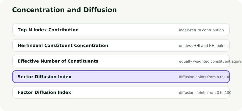
The family map prevents a category error. Contribution combines beginning weight and realized return. HHI and effective N inspect the weight vector before returns. Diffusion scores direction across a fixed component panel. Choosing the wrong branch may produce valid arithmetic that answers the wrong question.
Freeze the series identity
The selected formula is:
Classify each sector signal above tolerance as improving, within tolerance as unchanged, and below negative tolerance as deteriorating. One observation per declared sector, one signal definition and horizon, complete point-in-time coverage, and an explicit nonnegative tolerance. The relevant primary source establishes the underlying convention; the exact diagnostic, translated universe, and parameters remain package choices where stated.
The snapshot needs unique identifiers, finite values, complete coverage, and one point-in-time methodology. as_of is not enough in production: retain observation, availability, and knowledge times plus source owner, revision, and finality. A later corrected roster or classification must not overwrite what was knowable at the earlier cutoff.
Required input
| Field | Type | Unit and rule |
|---|---|---|
as_of | ISO date | common observation cutoff; retain availability and knowledge time separately |
component_id | string | one unique sector in the frozen taxonomy |
signal_change | finite number | decimal change for one declared signal, horizon, direction convention, and currency basis |
ready | boolean | false means sector coverage is incomplete |
tolerance | nonnegative number | decimal deadband; exact +/- tolerance is unchanged |
Output and refusal behavior
Return value from 0 to 100 plus improving, unchanged, deteriorating, and total counts. 50 is the arithmetic midpoint under 1/0.5/0 scoring, not an empirical forecast threshold.
The reference API uses strict comparisons and raises on incomplete panels. The lab exposes the same rule with live tolerance changes and a visible withheld state.
Read the mathematics, not only the score
A change greater than tolerance scores 1; a change less than negative tolerance scores 0; both equality boundaries and the entire deadband score 0.5. Every declared sector receives one equal vote.
0 <= D_sector <= 100and class counts sum toN.- Exact
+toleranceand-toleranceobservations are unchanged. - All unchanged sectors produce 50; equal improving and deteriorating counts with no unchanged sectors also produce 50.
- Missing sectors are not unchanged. Changing taxonomy, signal, horizon, direction, or tolerance starts a different series.
The output must travel with its series identity and diagnostic trace. A bare number strips away the universe, methodology, horizon, tolerance, and evidence status needed to interpret it.
Work the synthetic example
The following is labelled synthetic and all arithmetic is author-derived:
| Component | Signal change | Class | Score |
|---|---|---|---|
| Communication | 1.200% | improving | 1 |
| Consumer Discretionary | 0.800% | improving | 1 |
| Consumer Staples | 0.600% | improving | 1 |
| Energy | 0.400% | improving | 1 |
| Financials | 0.300% | improving | 1 |
| Health Care | 0.200% | unchanged | 0.5 |
| Industrials | 0.000% | unchanged | 0.5 |
| Materials | -0.200% | unchanged | 0.5 |
| Real Estate | -0.400% | deteriorating | 0 |
| Technology | -0.700% | deteriorating | 0 |
| Utilities | -1.000% | deteriorating | 0 |
The exact expected result is:
{
  "status": "resolved",
  "value": 59.09090909090909,
  "improving": 5,
  "unchanged": 3,
  "deteriorating": 3,
  "total": 11
}
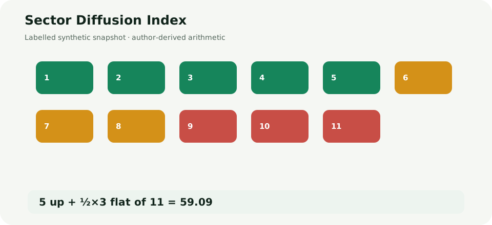
The visual keeps the distribution beside the aggregate. That matters because two identical aggregate values can conceal different component states. The values are synthetic teaching inputs; the displayed result is author-derived arithmetic.
Compare nearby methods
| Variant | Component vote | Best use | Main limitation |
|---|---|---|---|
| Equal-sector diffusion (selected) | each sector receives one 1/0.5/0 score | breadth independent of sector capitalization | a tiny sector has the same vote as a large sector |
| Capitalization-weighted sector breadth | weight each score by sector size | connect breadth to index economic weight | can reproduce headline concentration |
| Binary advance share | unchanged receives 0 rather than 0.5 | strict participation count | discontinuous around zero |
| Continuous average change | average raw sector changes | retain magnitude | no longer a diffusion index |
The comparison is part of the contract. A different numerator, denominator, component universe, weighting rule, tolerance, or signal horizon is not a cosmetic option—it defines a different series.
Implementation walkthrough
The reference algorithm validates before aggregating:
validate one complete fixed-taxonomy sector panel
validate one signal horizon and nonnegative tolerance
for each sector:
    if change > tolerance: score 1
    else if change < -tolerance: score 0
    else: score 0.5
diffusion = 100 * sum(scores) / sector_count
return value, class counts, and sector trace
Freeze the taxonomy and signal horizon, treat exact tolerance equality as unchanged, and reject a missing sector instead of renormalizing.
Python and TypeScript consume the same JSON fixture and return the same resolved fields. Invalid or incomplete input raises rather than being repaired. The playground deliberately translates its failure fixture into a visible withheld state because its job is to teach the refusal boundary.
Guided lab
Open the guided playground. Start from the informative canonical state, switch to Comparison, then Failure / boundary. Use Back and Step to inspect how each component enters the result. Change the tolerance and compare broad improvement, narrow deterioration, and incomplete sector coverage. Reset restores the exact canonical state, and reduced-motion Play advances one deterministic observation without starting a timer.
The calculation flow shows why point-in-time validation precedes aggregation.
Put the diagnostic into an operating workflow
Pair equal-sector diffusion with the cap-weighted headline return. Their disagreement answers whether a move is large because many sectors participate or because a few large sectors dominate.
A robust dashboard retains the input snapshot, formula version, parameters, component trace, and refusal reason. It should make methodology or taxonomy changes visible as breaks in series identity rather than quietly splicing them into history.
Edge cases and misuse boundaries
Do not mix sector taxonomies, count missing sectors as unchanged, or change the signal horizon between observations. Missing components are neither zero nor unchanged. A different roster, taxonomy, factor provider, share-class policy, currency, return basis, horizon, or tolerance defines a different series.
Main takeaway: Equal-sector diffusion measures participation, not the size of the market move.
Passing implementation tests proves that the code matches the selected definition. It does not prove association with future returns, usefulness after costs, causation, or suitability for an investment decision.
Evidence and historical boundary
The source records in REFERENCES.md establish only the claims mapped to them. They do not establish the synthetic numbers or silently define this package's translated universe and parameters.
A named historical case is deferred until a fixed licensed sector taxonomy, complete point-in-time sector signals, one horizon and tolerance, direction conventions, revision lineage, and redistribution permission. Deferral is a publication boundary, not a missing-data invitation: the public tutorial uses a transparent synthetic case rather than an irreproducible observed value.
Summary and handoff
You can now calculate D_{\mathrm{sector}}=100\frac{N_+ + 0.5N_0}{N}, identify the series-defining choices, interpret its edge regimes, preserve the audit trace, and reject incomplete snapshots. Continue with Factor Diffusion Index.
Primary sources and exact limitations are recorded in REFERENCES.md.
Rendered from the canonical Mermaid sources linked by this article.
Calculation Flow — Sector Diffusion Index
Purpose: validate series identity before producing the diagnostic.
Takeaway: Missing evidence is a state, never a zero contribution or neutral component.
ReferencesPrimary sources and evidence notesExpand the source trail, evidence role, and limitations behind the engineering choices.
Expand the source trail, evidence role, and limitations behind the engineering choices.
Claim-to-source map
| Material claim | Evidence | Classification |
|---|---|---|
| Diffusion can score increase/unchanged/decrease as 1/0.5/0 | TCB-DIFF | sourced transform |
| Equal sector votes and the 0.2% tolerance | definition contract | package application and parameter choice |
| Canonical values | datasets/canonical-fixture.json | synthetic input and author-derived calculation |
Every external source ID mapped above is expanded below. Provider or institutional conventions are not presented as universal laws; package translations and parameters remain labelled as implementation choices.
TCB-DIFF — How to Compute Diffusion Indexes
- Organization or authors: The Conference Board
- Source type: Institutional technical methodology
- Publication or effective date: 2012 technical-note convention
- Version: Web methodology accessed 2026-07-26
- URL or DOI: https://www.conference-board.org/data/bci/index.cfm?id=2180
- Accessed: 2026-07-26
- Jurisdiction: Global methodology unless the limitation states otherwise
- Supports: Diffusion scoring of 1 for increase, 0.5 for unchanged, 0 for decrease, divided by component count and multiplied by 100.
- Limitations: The source applies the convention to business-cycle components; sector and factor application here is an explicit package choice.
Full dependency-light reference implementations in both supported languages.
type Row = Record<string, unknown>;
const numberValue = (value: unknown, name: string): number => {
  if (typeof value !== "number" || !Number.isFinite(value)) throw new Error(`${name} must be a finite number`);
  return value;
};
const validateRows = (rows: Row[], weighted: boolean): void => {
  if (!rows.length) throw new Error("rows must not be empty");
  const seen = new Set<string>();
  for (const row of rows) {
    const key = row[weighted ? "security_id" : "component_id"];
    if (typeof key !== "string" || !key || seen.has(key)) throw new Error("component identifiers must be nonempty and unique");
    seen.add(key);
    if (row.ready === false) throw new Error("incomplete_component");
  }
};

export function calculate(rows: Row[], tolerance = 0.002) {
  validateRows(rows, false); tolerance=numberValue(tolerance,"tolerance");
  if (tolerance < 0) throw new Error("tolerance must be nonnegative");
  const changes=rows.map(row=>numberValue(row.signal_change,"signal_change"));
  const improving=changes.filter(x=>x>tolerance).length, deteriorating=changes.filter(x=>x < -tolerance).length, unchanged=rows.length-improving-deteriorating;
  return {status:"resolved", value:100*(improving+0.5*unchanged)/rows.length, improving, unchanged, deteriorating, total:rows.length};
}
The embedded lab now expands to its full document height, keeping the article as the only scroll surface.