Bayesian Change-Point Detection

State models are attractive because they turn a noisy sequence into an interpretable evolving belief. They are dangerous for exactly the same reason: a smooth line or decisive regime label can look like fact even when it is only the output of a fragile configuration. This tutorial shows how to maintain an online posterior over the time since the most recent change while keeping the information boundary and uncertainty visible.

The deliverable is practical. You will calculate one update, implement the recursion in Python and TypeScript, inspect eight model-specific scenarios, and use a guided lab to see why the state changes. The result is an educational filter, not an investment recommendation or a claim of predictive power.

The question this model answers

Bayesian Change-Point Detection answers a conditional question: given the selected model, its fixed configuration, and observations available through the current timestamp, what state summary should be carried forward?

That wording matters. It does not ask what the state “really was” after seeing the future. It does not estimate parameters. It does not decide whether a trading action is profitable. The run-length distribution is useful for monitoring possible structural shifts while making hazard and observation-model assumptions visible.

Intuition before notation

Every observation competes between continuing each existing run and starting a fresh run; the posterior retains uncertainty instead of returning one irreversible break. Every update therefore needs a ledger. The learner should be able to point to the prior, the prediction, the new evidence, and the posterior. If one of those pieces is hidden, the final curve becomes an assertion rather than an explanation.

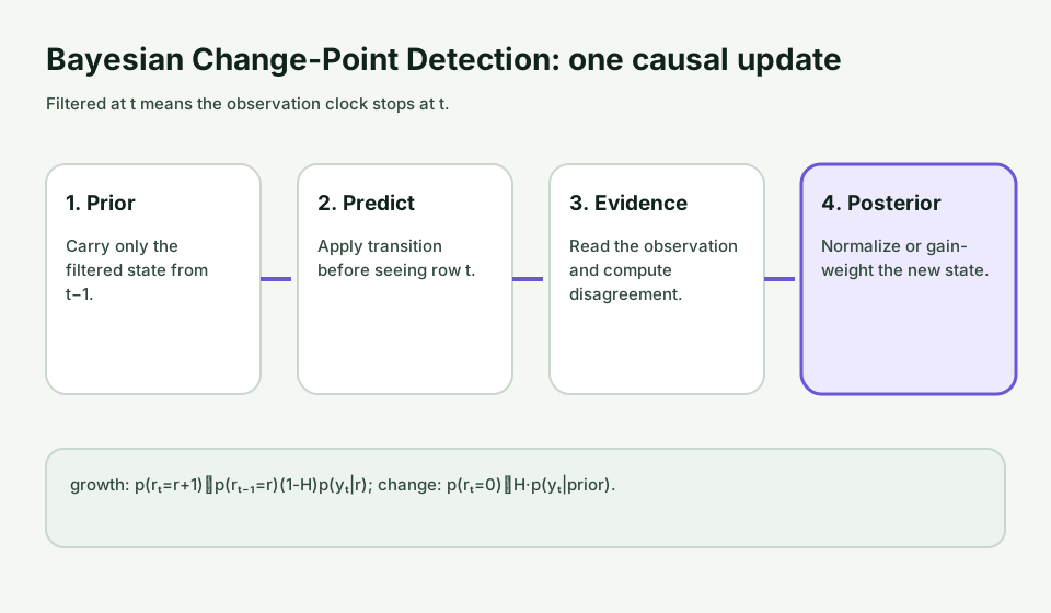
The state update visual is canonical: its labels correspond directly to the trace produced by both implementations.

The frozen definition

This article uses a known-variance constant-hazard online run-length filter. Constant-hazard BOCPD with a Gaussian observation model, known observation variance, normal prior on the segment mean, and a pre-observation change convention.

The core recursion is:

growth: p(rₜ=r+1)∝p(rₜ₋₁=r)(1-H)p(yₜ|r); change: p(rₜ=0)∝H·p(yₜ|prior).

The package excludes unknown-variance student-t prediction, offline segmentation, pruning approximations, learned hazards, and automatic trade triggers. Those are legitimate extensions, but adding them silently would make the arithmetic and information set ambiguous.

The package convention that changes the answer

This package uses a pre-observation reset: if a change occurs at t, y_t is scored under the fresh prior predictive and belongs to the new run. Sources or libraries that attach y_t to the ending run use a shifted run-length convention.

That sentence belongs beside the formula because two implementations can both be called Bayesian Change-Point Detection and still disagree when they initialize, index, or parameterize the recursion differently.

When this model is the right abstraction

Use BOCPD when uncertainty about time since the latest abrupt change is the target. Use an HMM or MSAR when recurring named states and transition memory are part of the model.

A high one-row change probability is an alarm under the model, not proof of a durable structural break. The practical selection test is not which curve looks smoothest. It is which latent representation, observation model, and information clock match the decision you must audit.

Filtering is not smoothing

A filtered state at t conditions on observations through t. A smoothed state at t can use later observations. Current statsmodels state-space documentation makes the same distinction between filtered and smoothed output (statsmodels 0.14.6 state-space guide).

For an online dashboard, alert, or causal backtest, silently substituting smoothed probabilities is a future-information leak. A retrospective research chart may use smoothing, but it must say so.

Inputs and clocks

The fixture uses 160 daily UTC observations per scenario. They are deterministic and synthetic. The timestamps are observation and availability times together; no exchange calendar, revision process, or vendor feed is implied.

The latent truth or true regime appears only for evaluation. The filter receives the observation values and fixed configuration. This separation lets us ask whether the recursion detects the generator without giving it the answer.

The configuration is part of the claim

{
  "hazard": 0.025,
  "observation_variance": 0.36,
  "prior_mean": 0.0,
  "prior_variance": 4.0
}

These values are implementation choices, not fitted estimates. A production claim would need a pre-declared fitting sample, likelihood or loss, optimizer, parameter constraints, model-selection process, and out-of-sample evaluation.

One update by hand

The first canonical observation is -0.32750535. Applying the published recursion gives change probability = 0.02500, map run length = 1, expected run length = 0.97500, active hypotheses = 2, map mean = -0.30046.

The calculation retains full precision and rounds only for display. The validator repeats this first update independently rather than asking the Python implementation to grade itself.

What the state ledger reveals

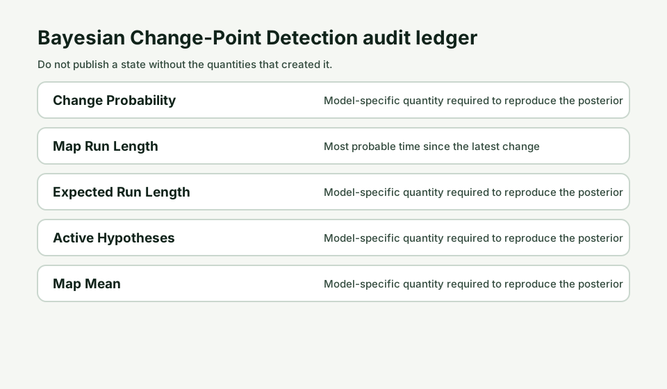
For this topic, the most useful fields are change probability, map run length, expected run length, active hypotheses, map mean. Read them together. A posterior without its predicted state hides persistence; a posterior without its innovation or likelihood hides the observation's contribution.

Eight scenarios that target this algorithm

The scenarios are not a generic family checklist. Each one changes a specific assumption that matters to Bayesian Change-Point Detection:

• Single clean break: One persistent mean shift at row 80 provides the control. The lab asks: When does change probability cross the declared threshold?
• Two breaks: Two persistent changes test repeated reset and recovery. The lab asks: Does the run-length posterior restart at both known changes?
• Recurring levels: Several returns to earlier levels test repeated detection. The lab asks: Does returning to an old level still count as a new segment?
• Small break: A subtle persistent shift competes with observation noise. The lab asks: How does evidence accumulate when no single row is decisive?
• Gradual drift: A smooth trend violates the abrupt-change assumption. The lab asks: Can the detector remain quiet even while its abrupt-change model is wrong?
• High noise: The observation model understates the generator noise. The lab asks: How many false alarms appear when variance is stale?
• Single outlier: One extreme row creates strong but nonpersistent change evidence. The lab asks: Can the diagnostic distinguish an alarm from a durable break?
• Short-lived level: A five-row level shift sits between an outlier and a new segment. The lab asks: How does hazard choice change the treatment of a temporary regime?

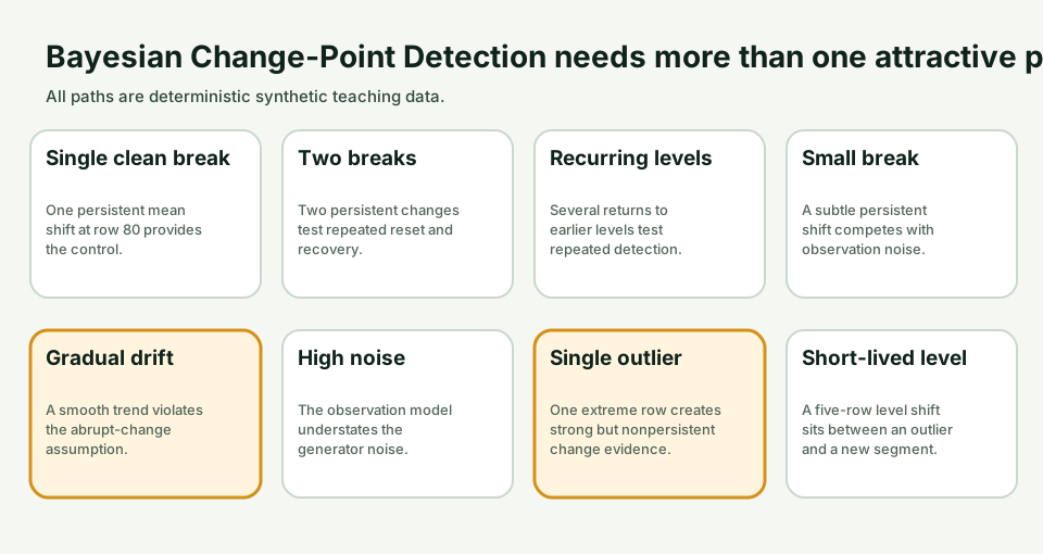
This is the difference between a demo and a learning reference: the reader can name the stressed assumption before looking at the output.

The algorithm

1. Validate observations and the fixed configuration.
2. Initialize the declared prior.
3. Predict before reading the current observation.
4. score the observation under the predicted state or hypotheses.
5. update and normalize.
6. record diagnostics and carry the filtered state forward.

This order is causal. Reordering it can leak the observation into the prior or apply the transition twice.

A diagnostic that can disagree with the picture

Inspect the full run-length posterior, declare an alarm threshold before looking at results, and compare alarms with known synthetic changes, delay, and false alarms.

The fixture-backed diagnostic is detection delay, false alarms, and the outlier trap. A fixed 0.5 teaching threshold is evaluated against known synthetic change rows; alarms, delay, false alarms, and log predictive density remain diagnostics rather than trading rules.

For the canonical full path, the published values include alarm threshold 0.5000, detected change count 1, mean detection delay rows 0.0000, false alarm count 0, maximum change probability 0.6380, maximum change index 80, mean log predictive density -0.6510. They are author-derived from known synthetic truth after the causal trace is complete. They are not an empirical result and do not establish usefulness on market data.

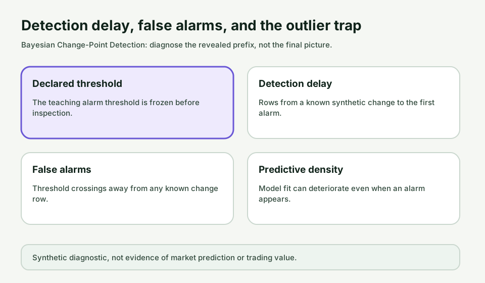
The interactive version recalculates the same quantities only over rows revealed through the current step. That makes the score informative without letting future truth influence an earlier filter state.

Python and TypeScript parity

Both implementations accept the same observation list and configuration object. Both return one trace row per observation. The shared JSON fixture compares every primary state field at a tolerance of 1e-9.

Readable reference arithmetic is intentional. Optimization comes after the contract is proved. In production, use stable matrix decompositions, monitored conditioning, and explicit schema/version controls appropriate to the chosen extension.

The model-specific audit discipline

Continuous-state filters must keep covariance nonnegative. Discrete-state filters must keep probabilities normalized. The UKF must publish its sigma-point weights. BOCPD must define whether a change occurs before or after the current observation. MSAR must define transition direction and which regime owns each AR coefficient.

These are not cosmetic implementation details. They determine the answer.

For this topic, the decisive audit is: Inspect the full run-length posterior, declare an alarm threshold before looking at results, and compare alarms with known synthetic changes, delay, and false alarms.

The outlier trap

A single extreme observation can produce a large innovation, strong emission ratio, or elevated change probability. That evidence is not the same as a persistent break. Compare the next several observations before attaching a narrative.

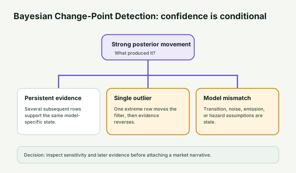
The failure map is a decision aid: check model assumptions, sensitivity, and subsequent evidence before treating a filtered state as operational truth.

Weak separation is an honest result

When regimes have similar emissions or observation noise dominates state movement, posterior probabilities should remain mixed. Forcing a hard label throws away the most important output: the model is uncertain.

The same principle applies to continuous filters. A narrow covariance is only meaningful if process and measurement variances are credible.

Historical evidence decision

The historical-example decision is not useful. A named market episode would add narrative appeal but would not validate a frozen latent-state model. The package therefore uses deterministic synthetic data so the hidden truth, observation clock, and state transition are auditable. A historical case would require licensed point-in-time observations, a parameter-estimation cutoff, revision policy, benchmark, and redistribution permission.

This avoids an especially common error: showing one named episode, fitting or tuning with knowledge of the whole episode, and then presenting a hindsight state chart as causal detection evidence.

Explore the guided lab

The self-contained playground implements choose → step → observe → explain → compare. Change the scenario and one meaningful parameter, then watch the trace, chart, guidance, and audit table recompute together.

Reset restores the canonical first row. Step and Play share one transition. In reduced-motion mode, Play advances exactly one observation and never starts a timer.

How to validate a production extension

• Freeze the information clock and revision policy.
• Separate fitting, filtering, forecasting, smoothing, and decision evaluation.
• Use time-ordered holdouts or rolling origins.
• Benchmark against a simpler state or regime rule.
• Test parameter sensitivity and transition/emission misspecification.
• Monitor numerical conditioning and probability normalization.
• Keep uncertainty visible in the user interface.
• Never convert a latent-state estimate directly into a performance claim.

Family map

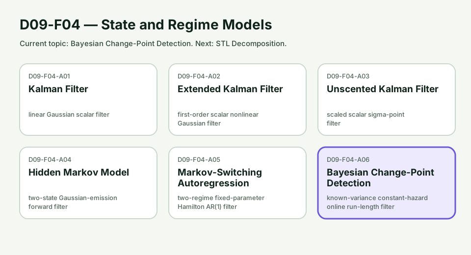
The next tutorial is STL Decomposition. The representation changes, but the audit question stays constant: exactly what did the model know when it produced this state?

Summary

You can now implement and audit Bayesian Change-Point Detection under a precise selected contract. The essential skill is not drawing a smooth state line. It is preserving the prior, prediction, evidence, posterior, and information boundary so another analyst can reproduce the result and challenge the assumptions.

Primary methodological records: Bayesian Online Changepoint Detection, Strictly Proper Scoring Rules, Prediction, and Estimation. The complete source-role and limitation ledger is in the canonical package.