
 By Islam Baraka
The useful outcome
AutoReg is the cleanest bridge from lag diagnostics to an executable forecast. It makes persistence, mean reversion, recursive substitution, and stability risk visible without mixing in latent innovations. The practical goal is a path that another person can reproduce from a declared cutoff—not a line whose origin, state, or future assumptions are hidden.
The question this tutorial answers is: How does an autoregression turn a fixed set of lag coefficients into an auditable multi-step conditional mean?
What you will build
You will calculate the model by hand, implement it in Python and TypeScript, inspect eight long synthetic scenarios, and learn where correct recursion ends and empirical forecast validation begins.
ACF and PACF are useful for lag diagnosis. Ordinary least squares helps explain estimation, but this package begins after coefficients have been frozen.
Freeze the variant before fitting anything
Fixed-coefficient AR(p) with an intercept, contiguous lags 1 through p, recursive point forecasts, and no exogenous or seasonal terms.
| Variant | Definition | Best use | Main limitation |
|---|---|---|---|
| Selected fixed AR(p) | coefficients supplied; recursive conditional mean | audit and teaching | does not estimate coefficients |
| AutoReg OLS | estimate c and lag coefficients by conditional OLS | fitting an AR-X model | sample and deterministic-term choices matter |
| Yule-Walker AR | match autocovariances | stationary AR estimation | not identical to conditional OLS |
| AR-X | add known exogenous regressors | driver-aware forecasting | future regressor path required |
This matters because forecast libraries often share a model-family name while differing in constants, trend representations, signs, initialization, missing data, or optimizer behavior.
Intuition before notation
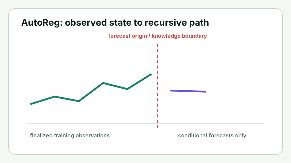
The first forecast uses observed lags. Every later forecast replaces an unavailable future lag with the forecast already produced for that time. The hardest part is observed lags versus recursively substituted forecast lags. The forecast origin is therefore a visible data boundary, not just the point where a chart changes color.
Formula and symbols
| Symbol | Meaning | Unit or range |
|---|---|---|
| p | autoregressive order | positive integer |
| c | intercept in the conditional-mean equation | series units |
| phi_i | coefficient on lag i | dimensionless |
| T | last available observation index | index |
| h | forecast horizon | 1 through H |
The formula is a conditional point forecast. Future random innovations use zero because zero is their conditional expectation—not because the future is known to contain no shocks.
Data that the formula is allowed to see
A finalized, equally spaced numeric series; ordered AR coefficients; an intercept in series units; and a positive integer horizon. Observations must be equally spaced, finite, ordered, and on one consistent scale. The model version and cutoff are frozen before the holdout. Revisions require a new forecast version rather than silent history replacement.
Algorithm
- Validate one finite, ordered, equally spaced series and p historical lags.
- For each in-sample eligible index, calculate the one-step conditional mean and residual.
- Copy the observed history into forecast state.
- For horizon one through H, apply the same AR equation and append the forecast.
- Publish coefficients, last lag state, forecast origin, and horizon with the path.
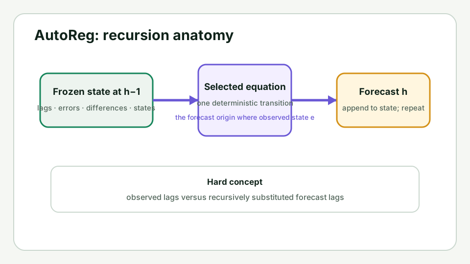
Hand calculation
The following is author-derived arithmetic over synthetic values:
{
  "values": [
    10,
    12,
    11
  ],
  "config": {
    "ar": [
      0.5
    ],
    "intercept": 5,
    "horizon": 2
  }
}
- h=1: 5 + 0.5(11) = 10.5
- h=2: 5 + 0.5(10.5) = 10.25
The expected path is [10.5, 10.25]. Independent tests pin
these values before the larger fixtures are generated.
Calculation flow
The order matters. Revealed actuals may score the path, but they may not alter the version that was issued at the cutoff.
Guided experiment
The standalone lab contains eight scenarios and 1,440 calendar-month-end observations. It trains on 144 values and forecasts a 36-value holdout. Start at horizon one, predict what state should persist, then Step through twelve model-specific checkpoints. Change the principal parameter and watch the complete path recompute from the frozen training data.
The scenarios isolate persistence, mean reversion, linear trend, seasonal structure, a late level shift, one gross outlier, a variance-regime change, and seasonal phase/amplitude drift. They are not selected trades or provider histories.
The state an expert audits
For this model, keep the ordered AR lag stack, the count of model-generated lags, and the intercept-implied mean visible.
Use a fixed AR recursion as a transparent baseline when lagged levels are the intended state. Before deployment, inspect stability, residual autocorrelation, structural breaks, and performance against a naïve forecast at every required horizon.
If the path drifts toward an implausible level, calculate c/(1-sum(phi)) before changing code. If early horizons look good but later ones collapse, inspect the characteristic roots and recursive substitution rather than adding arbitrary trend.
When implementations disagree, use this order: Two AR systems most often disagree because one treats c as an equation intercept while another reports a long-run mean, or because lag ordering, deterministic trend, estimation window, or missing timestamps differ.
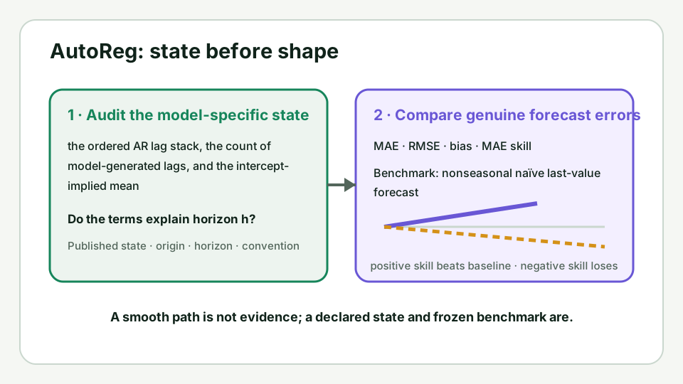
The workbench is deliberately quantitative. It connects the model's unique state to the declared benchmark rather than asking the learner to judge whether the purple line “looks right.”
Failure diagnosis
- A coefficient vector is not an order-selection result.
- Explosive or near-unit-root coefficients can create unstable long-horizon paths.
- Changing the intercept convention changes the implied long-run mean.
- Irregular timestamps or silent missing-value compression invalidate the lag meaning.
- Recursive forecasts accumulate model error even when arithmetic is exact.
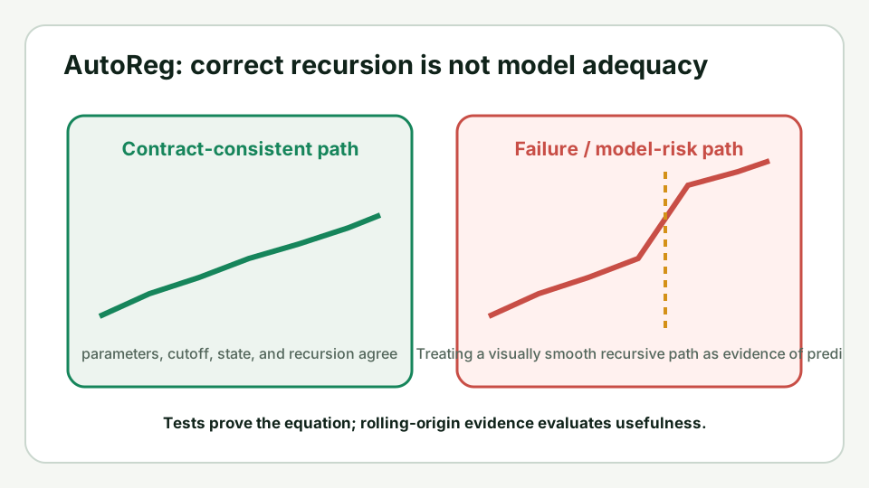
Treating a visually smooth recursive path as evidence of predictive or trading value. Correct arithmetic answers “did we implement the selected model?” It does not answer “is this a good model for this series?”
Implementation contract
The Python reference favors readable state transitions. TypeScript implements
the same contract independently. Shared fixtures and focused tests require
matching numeric paths within 1e-9 and exact agreement on lengths, nulls,
states, and invalid-input behavior.
Estimation is intentionally outside the public function. In a real workflow, fit or select parameters using only training data, record the method and version, pass the frozen result into this recursion engine, and evaluate using rolling origins against simple benchmarks.
Practical evaluation
Use a loss function that matches the decision, report by horizon, and include baseline forecasts. Preserve the refit schedule and origin timestamps. If prediction intervals are needed, choose and validate an uncertainty model; do not manufacture intervals from point forecasts alone.
The lab's declared baseline is nonseasonal naïve last-value forecast. At active horizon k,
it calculates errors only for the first k revealed holdout values:
MAE = mean(abs(actual - forecast));RMSE = sqrt(mean((actual - forecast)^2));bias = mean(actual - forecast);MAE skill = 1 - model_MAE / benchmark_MAE.
Positive skill means the model's revealed-prefix MAE is lower than the frozen benchmark's. Negative skill is useful evidence: the sophisticated recursion is losing to a simple rule on this synthetic path. When benchmark MAE is zero, skill is undefined rather than infinite. One origin still cannot establish general performance; repeat the complete procedure over rolling origins before making an empirical claim.
Related methods
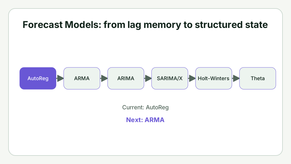
AutoReg introduces lag memory. ARMA adds innovation memory. ARIMA changes the modeled scale through differencing. SARIMA/SARIMAX adds seasonal polynomials and future driver scenarios. Holt-Winters maintains level, trend, and seasonal states directly. Theta combines a smoothed level with constrained drift.
Next: ARMA.
Historical and evidence boundary
A historical example is not useful for this mechanism lesson. A defensible case requires licensed point-in-time observations, identity, frequency, adjustment and revision basis, cutoff, parameters frozen before inspection, benchmark, holdout, and publication rights.
This tutorial establishes definition fidelity. It does not establish stationarity, model adequacy, forecast calibration, historical association, causation, profitability, or investment suitability.
Primary references
- statsmodels.tsa.ar_model.AutoReg — AutoReg is an AR-X(p) model estimated by conditional maximum likelihood using OLS and can include deterministic or exogenous terms.
- Forecasting: Principles and Practice — ARIMA models — ARIMA notation, differencing, AR and MA orders, stationarity/invertibility, and recursive point forecasting with future errors set to zero.
- Forecasting: Principles and Practice — Evaluating point forecast accuracy — Forecast accuracy must be measured on genuine forecasts outside the training sample; MAE, RMSE, scaled errors, and benchmarks answer different evaluation questions.
- Forecasting: Principles and Practice — Time series cross-validation — Rolling forecasting origins preserve temporal order and can evaluate horizon-specific errors without using future observations.
- Forecasting: Principles and Practice — Evaluating regression and residual behavior — Residual plots and residual autocorrelation diagnose information left in the fitted model, but residual size is not a substitute for genuine forecast error.
Rendered from the canonical Mermaid sources linked by this article.
AutoReg Calculation Flow
Purpose: separate validated historical state, fixed model parameters, recursive forecast state, and holdout evaluation.
Takeaway: evaluation data follows publication; it never repairs the already issued forecast.
ReferencesPrimary sources and evidence notesExpand the source trail, evidence role, and limitations behind the engineering choices.
Expand the source trail, evidence role, and limitations behind the engineering choices.
STATSMODELS_AUTOREG — statsmodels.tsa.ar_model.AutoReg
- Organization or authors: statsmodels developers
- Source type: Maintained official library documentation
- Publication or effective date: 2025-12-05 documentation build
- Version: statsmodels 0.14.6
- URL or DOI: https://www.statsmodels.org/stable/generated/statsmodels.tsa.ar_model.AutoReg.html
- Accessed: 2026-07-27
- Jurisdiction: Technical method; no legal jurisdiction.
- Supports: AutoReg is an AR-X(p) model estimated by conditional maximum likelihood using OLS and can include deterministic or exogenous terms.
- Limitations: The package teaches fixed-coefficient recursion and does not reproduce statsmodels estimation or trend conventions.
- Evidence role: Definition/variant comparison only; not provider data or an empirical result for the synthetic fixtures.
- Publication boundary: Link and paraphrase are public; no source dataset or copyrighted table is reproduced.
FPP_ARIMA — Forecasting: Principles and Practice — ARIMA models
- Organization or authors: Rob J. Hyndman and George Athanasopoulos
- Source type: Authoritative open forecasting textbook
- Publication or effective date: 2021 third edition; online version updated 2026-03-09
- Version: 3rd edition
- URL or DOI: https://otexts.com/fpp3/non-seasonal-arima.html
- Accessed: 2026-07-27
- Jurisdiction: Technical method; no legal jurisdiction.
- Supports: ARIMA notation, differencing, AR and MA orders, stationarity/invertibility, and recursive point forecasting with future errors set to zero.
- Limitations: Examples use the fable ecosystem; package-specific initialization remains an implementation choice.
- Evidence role: Definition/variant comparison only; not provider data or an empirical result for the synthetic fixtures.
- Publication boundary: Link and paraphrase are public; no source dataset or copyrighted table is reproduced.
FPP_ACCURACY — Forecasting: Principles and Practice — Evaluating point forecast accuracy
- Organization or authors: Rob J. Hyndman and George Athanasopoulos
- Source type: Authoritative open forecasting textbook
- Publication or effective date: 2021 third edition; online version updated 2026-03-09
- Version: 3rd edition
- URL or DOI: https://otexts.com/fpp3/accuracy.html
- Accessed: 2026-07-27
- Jurisdiction: Technical method; no legal jurisdiction.
- Supports: Forecast accuracy must be measured on genuine forecasts outside the training sample; MAE, RMSE, scaled errors, and benchmarks answer different evaluation questions.
- Limitations: A single synthetic holdout is a teaching comparison, not an empirical model-selection study.
- Evidence role: Definition/variant comparison only; not provider data or an empirical result for the synthetic fixtures.
- Publication boundary: Link and paraphrase are public; no source dataset or copyrighted table is reproduced.
FPP_TSCV — Forecasting: Principles and Practice — Time series cross-validation
- Organization or authors: Rob J. Hyndman and George Athanasopoulos
- Source type: Authoritative open forecasting textbook
- Publication or effective date: 2021 third edition; online version updated 2026-03-09
- Version: 3rd edition
- URL or DOI: https://otexts.com/fpp3/tscv.html
- Accessed: 2026-07-27
- Jurisdiction: Technical method; no legal jurisdiction.
- Supports: Rolling forecasting origins preserve temporal order and can evaluate horizon-specific errors without using future observations.
- Limitations: This family demonstrates one frozen origin; production claims require many origins and a declared refit schedule.
- Evidence role: Definition/variant comparison only; not provider data or an empirical result for the synthetic fixtures.
- Publication boundary: Link and paraphrase are public; no source dataset or copyrighted table is reproduced.
FPP_RESIDUALS — Forecasting: Principles and Practice — Evaluating regression and residual behavior
- Organization or authors: Rob J. Hyndman and George Athanasopoulos
- Source type: Authoritative open forecasting textbook
- Publication or effective date: 2021 third edition; online version updated 2026-03-09
- Version: 3rd edition
- URL or DOI: https://otexts.com/fpp3/regression-evaluation.html
- Accessed: 2026-07-27
- Jurisdiction: Technical method; no legal jurisdiction.
- Supports: Residual plots and residual autocorrelation diagnose information left in the fitted model, but residual size is not a substitute for genuine forecast error.
- Limitations: Residual diagnostics do not prove unbiasedness, calibrated intervals, or out-of-sample usefulness for these fixed teaching configurations.
- Evidence role: Definition/variant comparison only; not provider data or an empirical result for the synthetic fixtures.
- Publication boundary: Link and paraphrase are public; no source dataset or copyrighted table is reproduced.
Full dependency-light reference implementations in both supported languages.
type ForecastResult = {
  forecast:number[];
  fitted:(number|null)[];
  residuals?:number[];
  state:Record<string,unknown>;
  [key:string]:unknown;
};
const finite=(value:number,name:string)=>{
  if(typeof value!=="number"||!Number.isFinite(value))throw new Error(`${name} must be finite`);
  return value;
};
const positiveInt=(value:number,name:string,min=1)=>{
  if(!Number.isInteger(value)||value<min)throw new Error(`${name} must be an integer >= ${min}`);
  return value;
};
const series=(values:number[],minimum=2)=>{
  if(!Array.isArray(values)||values.length<minimum)throw new Error(`values must contain at least ${minimum} observations`);
  return values.map((value,index)=>finite(value,`values[${index}]`));
};
const coefficients=(values:number[],name:string,allowEmpty=true)=>{
  if(!Array.isArray(values)||(!allowEmpty&&values.length===0))throw new Error(`${name} must be a coefficient list`);
  return values.map((value,index)=>finite(value,`${name}[${index}]`));
};

export function forecastAutoReg(values:number[],ar:number[],intercept:number,horizon:number):ForecastResult{
  const a=coefficients(ar,"ar",false),p=a.length,y=series(values,p+1),c=finite(intercept,"intercept"),H=positiveInt(horizon,"horizon");
  const fitted:(number|null)[]=Array(p).fill(null),residuals:(number|null)[]=Array(p).fill(null);
  for(let t=p;t<y.length;t++){
    let prediction=c;for(let lag=1;lag<=p;lag++)prediction+=a[lag-1]*y[t-lag];
    fitted.push(prediction);residuals.push(y[t]-prediction);
  }
  const extended=[...y],forecast:number[]=[];
  for(let step=0;step<H;step++){
    let prediction=c;for(let lag=1;lag<=p;lag++)prediction+=a[lag-1]*extended[extended.length-lag];
    extended.push(prediction);forecast.push(prediction);
  }
  return {forecast,fitted,residuals,state:{order:p,last_values:y.slice(-p)}};
}
The embedded lab now expands to its full document height, keeping the article as the only scroll surface.