Ljung-Box

Two analysts can run “the same” time-series diagnostic and obtain different answers without either making an arithmetic error. One centered an ACF with a common denominator; another used an adjusted denominator. One ADF regression included a trend; another included only a constant. The lesson is not to distrust diagnostics. It is to make the statistical question visible.

By the end, you will be able to aggregate residual autocorrelations through lag h into the Ljung-Box Q statistic, calculate degrees of freedom after subtracting fitted ARMA parameters, and explain why a changed result may reflect an analyst choice rather than a changed process.

The practical decision

Do residual autocorrelations through lag h jointly contradict a white-noise adequacy check? The method helps aggregate residual autocorrelations into a portmanteau statistic with explicit model degrees of freedom. It does not choose a position, forecast a return, or establish a causal mechanism.

Prerequisites and scope

Residuals, ACF, chi-square reference distributions, p-values, and fitted-model degrees of freedom.

This tutorial freezes {"alpha": 0.05, "lags": 12, "model_df": 0}. That choice is deliberately narrower than the alternatives documented by the official statsmodels Ljung-Box documentation. The source establishes library semantics; the fixture and displayed arithmetic are project-authored.

Start with the null and its direction

H0: residual autocorrelations through the selected lag are jointly zero under the chi-square approximation. That sentence belongs beside the chart because a decision word by itself invites overclaiming.

The comparison is strict. Equality with the configured boundary does not reject. This detail sounds small, but an untested <= in place of < changes a boundary result and can quietly split Python and TypeScript behavior.

Intuition before notation

Aggregate squared residual autocorrelations and account explicitly for fitted-model degrees of freedom.

The central mental model is: transform the same ordered sample, expose the intermediate evidence, normalize once under a declared convention, and only then apply the null-specific rule.

Formula and symbols

Q=n(n+2)\sum_{k=1}^{h}\frac{\hat\rho_k^2}{n-k},\quad Q\overset{a}{\sim}\chi^2_{h-m}

Symbol	Meaning	Unit
`e_t`	ordered fitted-model residual	response unit
`rho_hat_k`	sample residual autocorrelation at lag k	unitless
`h`	maximum jointly tested lag	observations
`m`	fitted model degrees of freedom	parameter count
`Q`	Ljung-Box statistic	unitless
`df`	h-m chi-square reference degrees of freedom	count

Material variants

Variant	What changes	Main limitation
Ljung-Box (selected)	Uses n(n+2)/(n-k) finite-sample scaling.	Chi-square reference is asymptotic.
Box-Pierce	Uses n times the sum of squared autocorrelations.	Usually less accurate in smaller samples.
Model-adjusted df	Subtracts consumed ARMA parameters from h.	Incorrect model_df changes the p-value.
Seasonal lag selection	Includes lags aligned with a seasonal period.	Requires a declared period and selection rule.

These variants are not spelling differences. They can change finite-sample values, reference distributions, and interpretation.

Rendering system map…

Walk the deterministic known-DGP fixture

Synthetic teaching input: the canonical white-noise scenario contains 96 deterministic observations. For the 96-point white-noise residual fixture at h=12 and model_df=0, Q = 11.395764 with 12 degrees of freedom. The independently checked upper-tail probability is 0.495340, so the package fails to reject the joint zero-autocorrelation null.

The reference implementation returns 11.395764 and state fail-to-reject-residual-whiteness. An independent NumPy/SciPy route reproduces the checkpoint without importing either reference implementation.

What to notice in the calculation visual: every displayed number is either a parameter, an intermediate author-derived value, or the final bounded state.

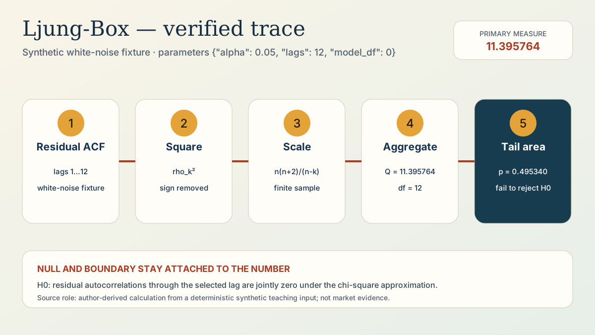
Ljung-Box verified calculation trace

Open the full-size calculation visual.

Implementation walkthrough

The Python and TypeScript references follow the same explicit stages:

Plain text

validate residual vector and h > model_df
compute centered unadjusted residual ACF through h
Q = n(n+2) * sum(rho_k^2/(n-k))
df = h-model_df
p_value = upper_tail_chi_square(Q, df)
reject residual-whiteness null only when p_value < alpha

The APIs reject missing/non-finite input, impossible lag/trim settings, and singular states. They return intermediate terms for auditability instead of returning only a color or Boolean. The full family module is copied into each package intentionally so every tutorial is executable in isolation; the topic example calls only the selected method.

Testing the definition, not a screenshot

The canonical fixture is necessary but not sufficient. The family-scoped checks also cover:

malformed and too-short input;
the exact equality direction at the decision boundary;
translation and nonzero-scale invariance where the formula implies it;
a comparison scenario from another known generating process;
Python/TypeScript value, state, and reason parity;
an independent formula or OLS route.

Passing those checks proves implementation agreement with this contract. It does not prove that the diagnostic has economic value.

Compare nearby scenarios

The playground includes white noise, AR(1), AR(2), MA(1), seasonal AR(12), near-unit-root, random-walk, trend-stationary, and level-break cases. Each contains 96 points. That variety matters:

AR and MA cases separate gradual decay from an approximate cutoff.
Seasonal dependence can be invisible when the maximum lag is too short.
A near-unit-root process is stationary by construction but can still produce an inconclusive finite-sample test.
A deterministic trend can make a level-stationarity specification fail for the right reason.
A level break can distort a no-break unit-root diagnosis.

Use the guided scenario laboratory to change one data-generating process or parameter preset at a time.

Read disagreements before chasing certainty

ACF inspects individual lags; Ljung–Box aggregates a selected lag set into one model-adequacy test. A disagreement between diagnostics may be the useful finding: the data may be near a boundary, trend-stationary rather than level-stationary, structurally broken, or underpowered at this sample size.

Apply Ljung-Box to residuals after a declared model fit. A non-rejection does not establish independence, normality, constant variance, or forecasting value.

Failure modes and what the output cannot authorize

The result cannot prove independence, identify a causal mechanism, guarantee future stability, or justify a position. Window, lag, deterministic-term, and missing-data choices belong in the decision record. If those choices were selected after viewing results, treat the output as exploratory and validate on a later untouched window.

Look-ahead: selecting a window or break narrative after observing future values turns confirmation into exploration.
Revision: a revised macro series cannot be treated as the history available to an earlier decision.
Missing periods: dropping a timestamp changes which values are lag neighbors.
Multiple testing: trying many lags and reporting one attractive bar changes the error rate.
Nonlinearity: zero linear autocorrelation does not establish independence or constant variance.

Historical-example decision — not-useful

A named security or famous event would add story value without revealing the true statistical process. The synthetic cases are preferable because their order, integration, seasonality, and break are known before calculation. Original papers supply methodological context; they do not turn this fixture into empirical market evidence.

Summary and handoff

You can now inspect the declared variant, reproduce the intermediate evidence, apply the strict null rule, and identify specification sensitivity. Continue to Zivot-Andrews Break Test, which answers a different question rather than replacing this result.

Workflows

Rendered from the canonical Mermaid sources linked by this article.

Ljung-Box decision flow

Purpose: show the selected method’s exact calculation stages and the branch from arithmetic into bounded interpretation.

Rendering system map…

Takeaway: the result is valid only for the declared transform, parameters, null, and sample. The next method answers a different question.

ReferencesPrimary sources and evidence notes

Expand the source trail, evidence role, and limitations behind the engineering choices.

Last evidence review: 2026-07-27

SM-ACF — statsmodels.tsa.stattools.acf

Organization or authors: statsmodels developers
Source type: Official maintained technical documentation
Publication or effective date: 2025-12-05
Version: statsmodels 0.14.6
URL or DOI: https://www.statsmodels.org/stable/generated/statsmodels.tsa.stattools.acf.html
Accessed: 2026-07-27
Jurisdiction / applicability: Methodology is not jurisdiction-specific; software semantics apply to statsmodels 0.14.6.
Evidence role: Sourced fact for the method, null, estimator variants, or maintained-library semantics—not evidence for the synthetic fixture.
Supports: ACF lag-zero convention, adjusted versus unadjusted denominators, missing-value choices, and confidence-band caveats.
Limitations: This package implements a direct O(nh) estimator and one explicit missing-value policy; it does not reproduce every statsmodels option.
Publication boundary: Link and paraphrase only; no restricted data payload is republished.

LB-1978 — On a measure of lack of fit in time series models

Organization or authors: Greta M. Ljung and George E. P. Box
Source type: Original peer-reviewed paper
Publication or effective date: 1978
Version: Biometrika 65(2), DOI 10.1093/biomet/65.2.297
URL or DOI: https://doi.org/10.1093/biomet/65.2.297
Accessed: 2026-07-27
Jurisdiction / applicability: Methodology is not jurisdiction-specific; applicability is limited to the model and assumptions in the paper.
Evidence role: Sourced fact for the method, null, estimator variants, or maintained-library semantics—not evidence for the synthetic fixture.
Supports: Finite-sample-scaled portmanteau statistic for residual autocorrelation.
Limitations: The asymptotic approximation does not establish independence, model correctness, or predictive usefulness.
Publication boundary: Link and paraphrase only; no restricted data payload is republished.

SM-LB — statsmodels.stats.diagnostic.acorr_ljungbox

Organization or authors: statsmodels developers
Source type: Official maintained technical documentation
Publication or effective date: 2025-12-05
Version: statsmodels 0.14.6
URL or DOI: https://www.statsmodels.org/stable/generated/statsmodels.stats.diagnostic.acorr_ljungbox.html
Accessed: 2026-07-27
Jurisdiction / applicability: Methodology is not jurisdiction-specific; software semantics apply to statsmodels 0.14.6.
Evidence role: Sourced fact for the method, null, estimator variants, or maintained-library semantics—not evidence for the synthetic fixture.
Supports: Demeaning, lag conventions, model degrees of freedom, and chi-square p-value semantics.
Limitations: The package accepts one maximum lag and does not reproduce seasonal or automatic-lag options.
Publication boundary: Link and paraphrase only; no restricted data payload is republished.

Evidence decisions

Sourced fact: maintained documentation and original papers establish the method, null, and material variants.
Implementation choice: denominator, estimator, deterministic terms, lag/bandwidth, trim, and any critical boundary are frozen by this package.
Synthetic teaching input: all scenario values come from the archived deterministic generator; none is a provider observation.
Author-derived calculation: expected outputs and worked arithmetic are calculated from those synthetic inputs and independently checked.
Historical example — not-useful: a controlled known-DGP case reveals whether the diagnostic behaves as designed; a named market case cannot reveal the true process and would add selection and causal-storytelling risks.

Implementation

Full dependency-light reference implementations in both supported languages.

diagnostics.ts

export type DiagnosticResult = Record<string, unknown>;

const EPS = 1e-12;

function series(values: number[], minimum = 8): number[] {
  if (!Array.isArray(values) || values.length < minimum ||
      values.some((value) => !Number.isFinite(value))) {
    throw new Error(`values must contain at least ${minimum} finite observations`);
  }
  return values.map(Number);
}

function integer(name: string, value: number, low: number, high: number): number {
  if (!Number.isInteger(value) || value < low || value > high) {
    throw new Error(`${name} must be an integer in [${low}, ${high}]`);
  }
  return value;
}

function numberIn(name: string, value: number, low: number, high: number): number {
  if (!Number.isFinite(value) || value < low || value > high) {
    throw new Error(`${name} must be finite and in [${low}, ${high}]`);
  }
  return value;
}

export function acf(values: number[], maxLag = 12): DiagnosticResult {
  const x = series(values);
  integer("maxLag", maxLag, 1, x.length - 1);
  const mean = x.reduce((a, b) => a + b, 0) / x.length;
  const centered = x.map((value) => value - mean);
  const denominator = centered.reduce((sum, value) => sum + value * value, 0);
  if (denominator <= EPS) throw new Error("ACF is undefined for a constant series");
  const numerators = [denominator];
  const coefficients = [1];
  for (let lag = 1; lag <= maxLag; lag += 1) {
    let numerator = 0;
    for (let index = lag; index < x.length; index += 1) {
      numerator += centered[index] * centered[index - lag];
    }
    numerators.push(numerator);
    coefficients.push(numerator / denominator);
  }
  return {
    method: "acf", variant: "centered-unadjusted-direct", nobs: x.length,
    max_lag: maxLag, mean, denominator, numerators, coefficients,
    confidence_95: 1.96 / Math.sqrt(x.length), state: "estimated",
    reason: "finite centered series with nonzero variance",
  };
}

export function pacf(values: number[], maxLag = 12): DiagnosticResult {
  const x = series(values);
  integer("maxLag", maxLag, 1, Math.min(x.length - 1, Math.floor(x.length / 2)));
  const rho = acf(x, maxLag).coefficients as number[];
  const coefficients = [1, rho[1]];
  const recursion: Record<string, number>[] = [
    {lag: 1, reflection: rho[1], prediction_variance: 1 - rho[1] ** 2},
  ];
  let phi = [rho[1]];
  let innovation = 1 - rho[1] ** 2;
  if (innovation <= EPS) throw new Error("PACF recursion is singular at lag 1");
  for (let lag = 2; lag <= maxLag; lag += 1) {
    let numerator = rho[lag];
    for (let index = 1; index < lag; index += 1) {
      numerator -= phi[index - 1] * rho[lag - index];
    }
    const reflection = numerator / innovation;
    const updated = phi.map((value, index) => value - reflection * phi[lag - index - 2]);
    updated.push(reflection);
    innovation *= 1 - reflection ** 2;
    if (innovation <= EPS) throw new Error(`PACF prediction variance is nonpositive at lag ${lag}`);
    phi = updated;
    coefficients.push(reflection);
    recursion.push({lag, reflection, prediction_variance: innovation});
  }
  return {
    method: "pacf", variant: "biased-yule-walker-levinson-durbin",
    nobs: x.length, max_lag: maxLag, coefficients, acf_coefficients: rho,
    recursion, confidence_95: 1.96 / Math.sqrt(x.length), state: "estimated",
    reason: "positive prediction variance through requested lag",
  };
}

function inverse(matrix: number[][]): number[][] {
  const n = matrix.length;
  const a = matrix.map((row, i) => [...row, ...Array.from({length: n}, (_, j) => i === j ? 1 : 0)]);
  for (let column = 0; column < n; column += 1) {
    let pivot = column;
    for (let row = column + 1; row < n; row += 1) {
      if (Math.abs(a[row][column]) > Math.abs(a[pivot][column])) pivot = row;
    }
    if (Math.abs(a[pivot][column]) <= EPS) throw new Error("regression design is singular");
    [a[column], a[pivot]] = [a[pivot], a[column]];
    const scale = a[column][column];
    a[column] = a[column].map((value) => value / scale);
    for (let row = 0; row < n; row += 1) {
      if (row === column) continue;
      const factor = a[row][column];
      a[row] = a[row].map((value, j) => value - factor * a[column][j]);
    }
  }
  return a.map((row) => row.slice(n));
}

function ols(y: number[], design: number[][]) {
  const rows = design.length;
  const columns = design[0]?.length ?? 0;
  if (!rows || y.length !== rows || rows <= columns) throw new Error("invalid regression dimensions");
  const xtx = Array.from({length: columns}, (_, i) =>
    Array.from({length: columns}, (_, j) =>
      design.reduce((sum, row) => sum + row[i] * row[j], 0)));
  const xty = Array.from({length: columns}, (_, i) =>
    design.reduce((sum, row, r) => sum + row[i] * y[r], 0));
  const inv = inverse(xtx);
  const beta = inv.map((row) => row.reduce((sum, value, j) => sum + value * xty[j], 0));
  const residuals = y.map((actual, r) =>
    actual - design[r].reduce((sum, value, c) => sum + value * beta[c], 0));
  const sse = residuals.reduce((sum, value) => sum + value * value, 0);
  const df = rows - columns;
  const sigma2 = sse / df;
  const stderr = inv.map((row, index) => Math.sqrt(Math.max(0, sigma2 * row[index])));
  return {beta, stderr, residuals, sse, sigma2, df_resid: df, nobs: rows};
}

export function adf(values: number[], lags = 1, criticalValue = -2.86): DiagnosticResult {
  const x = series(values, 16);
  integer("lags", lags, 0, Math.min(12, Math.floor(x.length / 4)));
  numberIn("criticalValue", criticalValue, -20, -0.1);
  const differences = x.slice(1).map((value, index) => value - x[index]);
  const response: number[] = [];
  const design: number[][] = [];
  for (let time = lags + 1; time < x.length; time += 1) {
    response.push(differences[time - 1]);
    const laggedDifferences = Array.from({length: lags}, (_, index) =>
      differences[time - index - 2]);
    design.push([1, x[time - 1], ...laggedDifferences]);
  }
  const regression = ols(response, design);
  const statistic = regression.beta[1] / regression.stderr[1];
  const reject = statistic < criticalValue;
  return {
    method: "adf", variant: "constant-only-fixed-lag", nobs: x.length,
    regression_nobs: regression.nobs, lags, gamma: regression.beta[1],
    gamma_standard_error: regression.stderr[1], statistic,
    critical_value: criticalValue, reject_null: reject,
    state: reject ? "reject-unit-root" : "fail-to-reject-unit-root",
    reason: reject ? "statistic-below-boundary" : "statistic-not-below-boundary",
    coefficients: regression.beta, residual_sse: regression.sse, df_resid: regression.df_resid,
  };
}

export function kpss(values: number[], lags = 5, criticalValue = 0.463): DiagnosticResult {
  const x = series(values, 16);
  integer("lags", lags, 0, Math.min(12, x.length - 2));
  numberIn("criticalValue", criticalValue, 0.001, 10);
  const mean = x.reduce((a, b) => a + b, 0) / x.length;
  const residuals = x.map((value) => value - mean);
  let running = 0;
  const cumulative = residuals.map((value) => (running += value));
  const numerator = cumulative.reduce((sum, value) => sum + value * value, 0) / x.length ** 2;
  let longRunSum = residuals.reduce((sum, value) => sum + value * value, 0);
  const covarianceTerms: Record<string, number>[] = [];
  for (let lag = 1; lag <= lags; lag += 1) {
    let crossProduct = 0;
    for (let index = lag; index < x.length; index += 1) {
      crossProduct += residuals[index] * residuals[index - lag];
    }
    const weight = 1 - lag / (lags + 1);
    longRunSum += 2 * weight * crossProduct;
    covarianceTerms.push({lag, weight, cross_product: crossProduct});
  }
  const longRunVariance = longRunSum / x.length;
  if (longRunVariance <= EPS) throw new Error("KPSS long-run variance must be positive");
  const statistic = numerator / longRunVariance;
  const reject = statistic > criticalValue;
  return {
    method: "kpss", variant: "level-stationary-fixed-bartlett-bandwidth",
    nobs: x.length, lags, residual_mean: residuals.reduce((a, b) => a + b, 0) / x.length,
    partial_sum_numerator: numerator, long_run_variance: longRunVariance,
    covariance_terms: covarianceTerms, statistic, critical_value: criticalValue,
    reject_null: reject,
    state: reject ? "reject-level-stationarity" : "fail-to-reject-level-stationarity",
    reason: reject ? "statistic-above-boundary" : "statistic-not-above-boundary",
  };
}

function logGamma(value: number): number {
  const c = [0.99999999999980993, 676.5203681218851, -1259.1392167224028,
    771.32342877765313, -176.61502916214059, 12.507343278686905,
    -0.13857109526572012, 9.9843695780195716e-6, 1.5056327351493116e-7];
  if (value < 0.5) return Math.log(Math.PI) - Math.log(Math.sin(Math.PI * value)) - logGamma(1 - value);
  const z = value - 1;
  let total = c[0];
  for (let i = 1; i < c.length; i += 1) total += c[i] / (z + i);
  const t = z + 7.5;
  return 0.5 * Math.log(2 * Math.PI) + (z + 0.5) * Math.log(t) - t + Math.log(total);
}

function gammaQ(shape: number, value: number): number {
  if (value === 0) return 1;
  if (value < shape + 1) {
    let term = 1 / shape;
    let total = term;
    let ap = shape;
    for (let i = 0; i < 200; i += 1) {
      ap += 1; term *= value / ap; total += term;
      if (Math.abs(term) < Math.abs(total) * 1e-15) break;
    }
    const p = total * Math.exp(-value + shape * Math.log(value) - logGamma(shape));
    return Math.max(0, Math.min(1, 1 - p));
  }
  let b = value + 1 - shape;
  let c = 1 / 1e-300;
  let d = 1 / b;
  let h = d;
  for (let i = 1; i <= 200; i += 1) {
    const an = -i * (i - shape);
    b += 2; d = an * d + b; if (Math.abs(d) < 1e-300) d = 1e-300;
    c = b + an / c; if (Math.abs(c) < 1e-300) c = 1e-300;
    d = 1 / d;
    const delta = d * c; h *= delta;
    if (Math.abs(delta - 1) < 1e-15) break;
  }
  return Math.max(0, Math.min(1,
    Math.exp(-value + shape * Math.log(value) - logGamma(shape)) * h));
}

export function ljungBox(values: number[], lags = 12, modelDf = 0, alpha = 0.05): DiagnosticResult {
  const x = series(values, 16);
  integer("lags", lags, 1, Math.min(24, x.length - 1));
  integer("modelDf", modelDf, 0, lags - 1);
  numberIn("alpha", alpha, 0.0001, 0.5);
  const correlation = acf(x, lags).coefficients as number[];
  const terms = Array.from({length: lags}, (_, index) => {
    const lag = index + 1;
    return {lag, acf: correlation[lag], term: correlation[lag] ** 2 / (x.length - lag)};
  });
  const statistic = x.length * (x.length + 2) *
    terms.reduce((sum, item) => sum + item.term, 0);
  const degreesOfFreedom = lags - modelDf;
  const pValue = gammaQ(degreesOfFreedom / 2, statistic / 2);
  const reject = pValue < alpha;
  return {
    method: "ljung_box", variant: "demeaned-residual-portmanteau",
    nobs: x.length, lags, model_df: modelDf, degrees_of_freedom: degreesOfFreedom,
    terms, statistic, p_value: pValue, alpha, reject_null: reject,
    state: reject ? "reject-residual-whiteness" : "fail-to-reject-residual-whiteness",
    reason: reject ? "p-value-below-alpha" : "p-value-not-below-alpha",
  };
}

export function zivotAndrews(
  values: number[], lags = 1, trim = 0.15, criticalValue = -4.80,
): DiagnosticResult {
  const x = series(values, 32);
  integer("lags", lags, 0, Math.min(8, Math.floor(x.length / 6)));
  numberIn("trim", trim, 0.05, 0.30);
  numberIn("criticalValue", criticalValue, -20, -0.1);
  const differences = x.slice(1).map((value, index) => value - x[index]);
  const first = Math.max(lags + 3, Math.ceil(x.length * trim));
  const last = Math.min(x.length - lags - 3, Math.floor(x.length * (1 - trim)) - 1);
  const scan: Record<string, number>[] = [];
  for (let breakIndex = first; breakIndex <= last; breakIndex += 1) {
    const response: number[] = [];
    const design: number[][] = [];
    for (let time = lags + 1; time < x.length; time += 1) {
      response.push(differences[time - 1]);
      const lagged = Array.from({length: lags}, (_, index) => differences[time - index - 2]);
      design.push([1, time + 1, x[time - 1], time > breakIndex ? 1 : 0, ...lagged]);
    }
    const regression = ols(response, design);
    scan.push({
      break_index: breakIndex, statistic: regression.beta[2] / regression.stderr[2],
      gamma: regression.beta[2], gamma_standard_error: regression.stderr[2],
      level_shift: regression.beta[3], residual_sse: regression.sse,
    });
  }
  const selected = scan.reduce((best, item) =>
    item.statistic < best.statistic ? item : best);
  const reject = selected.statistic < criticalValue;
  return {
    method: "zivot_andrews", variant: "intercept-break-fixed-lag", nobs: x.length,
    lags, trim, candidate_start: first, candidate_end: last, scan,
    break_index: selected.break_index, statistic: selected.statistic,
    gamma: selected.gamma, gamma_standard_error: selected.gamma_standard_error,
    level_shift: selected.level_shift, critical_value: criticalValue,
    reject_null: reject,
    state: reject ? "reject-unit-root-with-break" : "fail-to-reject-unit-root-with-break",
    reason: reject ? "minimum-statistic-below-boundary" : "minimum-statistic-not-below-boundary",
  };
}

export function runDiagnostic(
  values: number[], method: string, params: Record<string, number> = {},
): DiagnosticResult {
  if (method === "acf") return acf(values, params.max_lag ?? 12);
  if (method === "pacf") return pacf(values, params.max_lag ?? 12);
  if (method === "adf") return adf(values, params.lags ?? 1, params.critical_value ?? -2.86);
  if (method === "kpss") return kpss(values, params.lags ?? 5, params.critical_value ?? 0.463);
  if (method === "ljung_box") return ljungBox(values, params.lags ?? 12, params.model_df ?? 0, params.alpha ?? 0.05);
  if (method === "zivot_andrews") return zivotAndrews(values, params.lags ?? 1, params.trim ?? 0.15, params.critical_value ?? -4.80);
  throw new Error(`unsupported diagnostic method: ${method}`);
}

Playground

The embedded lab now expands to its full document height, keeping the article as the only scroll surface.

Full-height labplaygroundOpen full screen