Trend, Seasonality, Cycles, and Remainder

Beginner level · synthetic teaching data · Python and TypeScript verification

The useful question

What does Trend, Seasonality, Cycles, and Remainder help us see, and what can it never prove by itself?

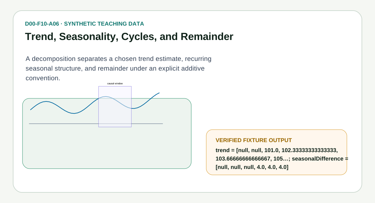
Three separate diagnostics read one series: a trailing moving-average trend, a period-over-period seasonal difference, and the remainder that is left once the trend is subtracted. This sounds compact because a statistic or model is compression: it keeps information relevant to one question and drops other detail. The first skill is therefore not memorizing notation. It is matching a human question to the information the method preserves.

For this package the frozen convention is trendₜ=mean(xₜ₋w₊₁…xₜ); seasonalDifferenceₜ=xₜ−xₜ₋ₚ; remainderₜ=xₜ−trendₜ. On the canonical synthetic fixture, the independently stored result is trend = [null, null, 101.0, 102.33333333333333, 103.66666666666667, 105.0]; seasonalDifference = [null, null, null, 4.0, 4.0, 4.0]; remainder = [null, null, 0.0, 1.6666666666666714, 2.3333333333333286, 0.0]; period = 3.

Begin with the picture

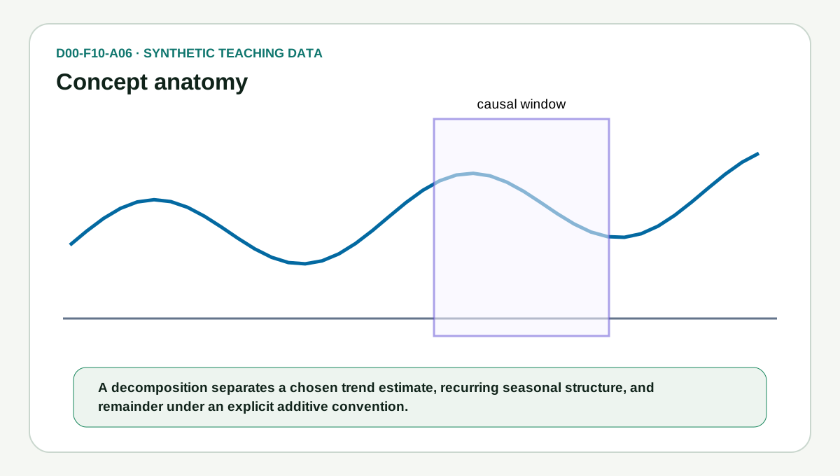
The visual keeps inputs, transformation, and output in separate layers. That separation is important in financial engineering. Raw observations have units, timestamps, identifiers, and availability rules. A derived number inherits those choices even when its final display looks simple.

Ask three questions while reading the picture:

1. Which observations are allowed to influence the result?
2. Which feature—magnitude, order, probability, time, path, or numerical precision—is preserved?
3. Which different datasets could produce the same output?

The third question reveals the method's blind spot. A summary can be correct and still be insufficient for a decision.

Translate the rule into plain language

trendₜ=mean(xₜ₋w₊₁…xₜ); seasonalDifferenceₜ=xₜ−xₜ₋ₚ; remainderₜ=xₜ−trendₜ

Read each symbol as a data instruction, not decoration. A sum declares which observations enter. A denominator declares the reference population or sample. A lag declares which information is earlier. A probability declares a model and support. A square, absolute value, rank, or quantile declares which differences matter. A tolerance declares when two floating-point outputs count as equivalent.

The package stores these decisions in DATA-CONTRACT.md so a future implementation cannot quietly adopt a library default that changes the answer.

The most important thing to say about these three lines is what they are not. They are three separate readings of the same series, not three pieces that add back up to it. Only one identity holds: xₜ = trendₜ + remainderₜ, wherever the trend is defined. The remainder is what is left after the trend is taken away, which means any seasonal swing is still sitting inside it. Calling it an irregular or noise term would be wrong.

seasonalDifference is a separate question, asked in a separate way: how does today compare with the same point one period ago? It is a change, not a component. You cannot subtract it from the remainder and call what is left irregular, and adding all three outputs together overshoots the observation by exactly seasonalDifferenceₜ. The fixture shows that plainly: at the fourth observation the trend is 102.33…, the remainder is 1.67, the seasonal difference is 4.0, and those sum to 108 against an actual value of 104.

There is also no cycle in the output, despite the topic's name. A cycle is the slow, irregular swing that is neither the long-run trend nor the fixed-length season, and isolating one requires a band-pass or state-space filter, an assumed cycle length, and a rule for what to do at the ends of the sample. That is a larger calculation than the one frozen here, and inventing a cycle field out of a moving average would be worse than leaving it out. What this topic can teach honestly is the vocabulary, the two diagnostics it does compute, and what a real decomposition would still need: seasonal indices averaged by position in the cycle, centred so they sum to zero, and then subtracted.

Work the synthetic example

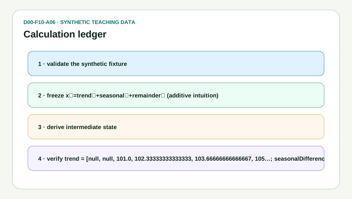
The fixture at ../examples/worked-example.json contains the exact input and expected fields. The verified output is trend = [null, null, 101.0, 102.33333333333333, 103.66666666666667, 105.0]; seasonalDifference = [null, null, null, 4.0, 4.0, 4.0]; remainder = [null, null, 0.0, 1.6666666666666714, 2.3333333333333286, 0.0]; period = 3. It is intentionally small enough to audit but not presented as a real market observation.

Use this five-step verification habit:

1. Confirm field names, units, array lengths, and timestamps.
2. Recalculate the first intermediate quantity by hand.
3. Apply the stated convention without early rounding.
4. Compare only after aligning output names and numerical tolerance.
5. Write one sentence that states both the result and its limitation.

The Python and TypeScript facades read the same fixture. Cross-language agreement is useful evidence that both implement the frozen rule, but it does not prove that the rule is suitable for every dataset.

What changes the answer?

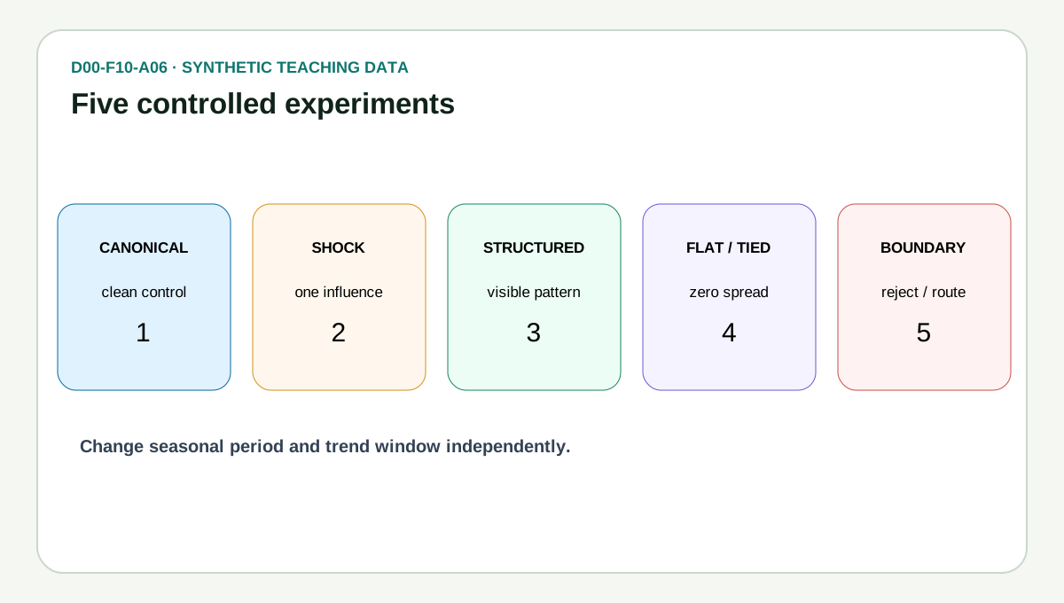
The guided lab includes 48 observations in five synthetic scenarios: canonical, one-shock, structured or symmetric, flat or tied, and boundary/failure. Each scenario changes one teaching feature while keeping the rest understandable.

Change seasonal period and trend window independently. Predict first. Then reveal observations with Step or Play and compare the diagnostic panel. Prediction makes the lab an experiment rather than a moving illustration.

The parameter control is family-specific. It changes spread for robust statistics, probability for event models, scale for distributions, visible sample size for inference, influence for regression, window length for time series, confidence for risk, or numerical tolerance for reproducibility.

The boundary is part of the answer

A moving average and seasonal difference are diagnostics, not a unique decomposition of the data-generating process.

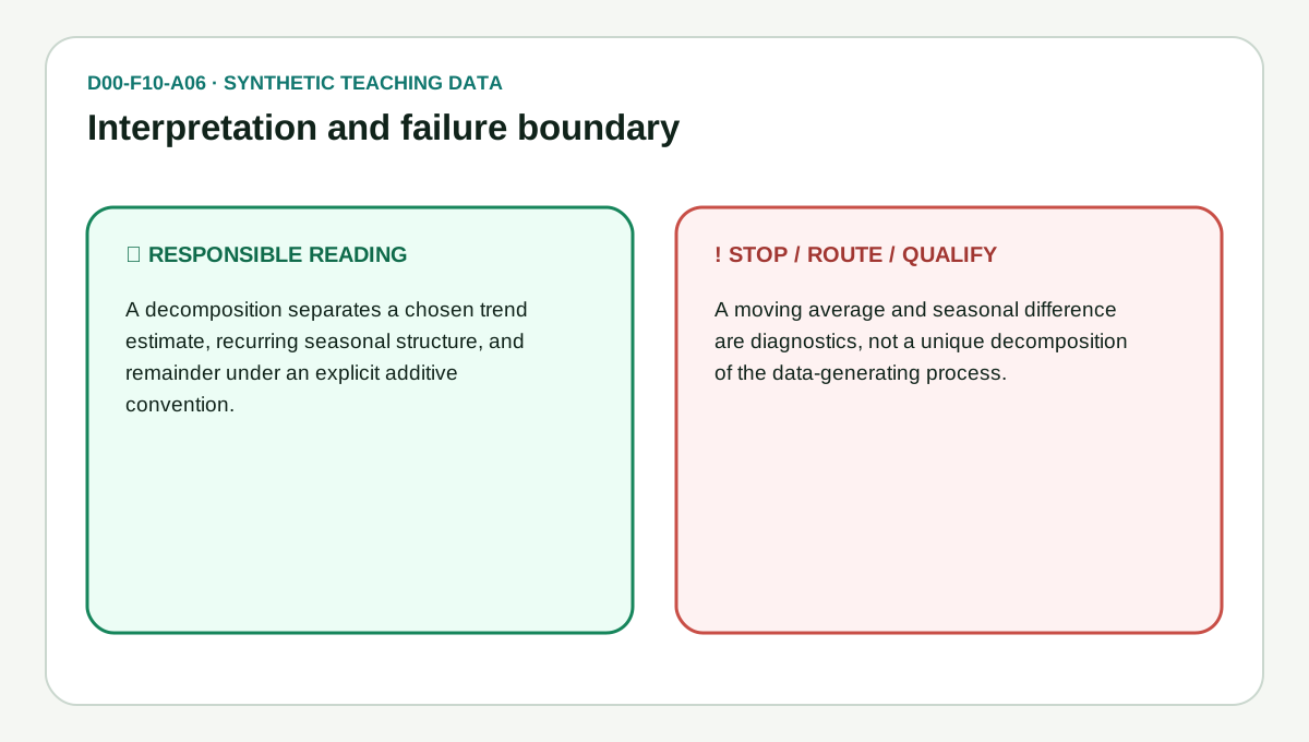
This is not a disclaimer added after the lesson. It is part of the mathematical contract. Undefined denominators, impossible probabilities, zero variance, invalid windows, future leakage, misaligned benchmarks, and unsupported numerical states should stop the calculation or route it to a different method.

A clean number does not establish causation or future performance. Passing an implementation fixture answers “Did we calculate the selected definition?” It does not answer “Will this signal remain useful after costs, bias controls, and new data?”

Nearby methods and selection logic

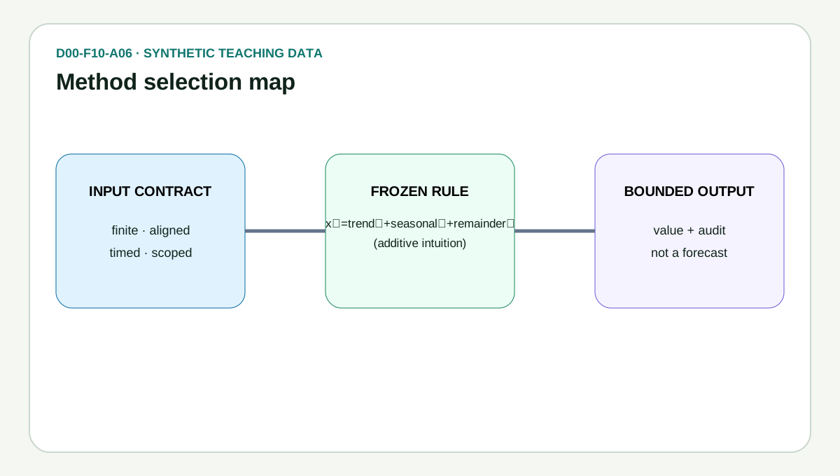
Choose the simplest method that preserves the feature your decision needs. Pair magnitude summaries with distribution views, probability models with assumption checks, estimates with uncertainty, correlations with scatterplots and subgroup analysis, time-series statistics with causal splits, risk ratios with paths and tail views, and numerical outputs with metadata and tolerance policies.

If two tools produce different answers, do not average them automatically. First ask whether they use different centers, denominators, tails, ranks, time windows, probability models, frequencies, or invalid-state rules.

Implementation walkthrough

The reference flow is deliberately readable:

validate required fields and alignment
freeze convention, time order, and parameter boundaries
derive intermediate state at full precision
calculate the named output
attach audit fields and reason codes
reject unsupported states

The narrow topic facade keeps the public function discoverable. Shared arithmetic prevents eighty foundational topics from drifting into eighty incompatible definitions. Optimization can come later; explicit state and testability come first.

Testing beyond the happy path

A responsible test set includes canonical arithmetic, equality boundaries, zero and constant states, malformed values, misalignment, numerical tolerance, and causal ordering where relevant. For models, it separates implementation correctness from model fit. For risk metrics, it freezes sign, confidence, horizon, and annualization. For reproducibility, it verifies reset, seed, version, and metadata behavior.

The browser playground adds another layer: controls must recompute immediately, Reset must be deterministic, Step and Play must share one transition, reduced-motion behavior must remain useful, and mobile layouts must not hide diagnostics.

A safe financial interpretation

Imagine the fixture represents validated returns, prices, durations, or model outputs. Before applying the formula, add currency, unit, calendar, corporate-action basis, observation time, availability time, source ownership, and missing-value policy. Without those fields, a mathematically correct result may describe the wrong economic object.

No result in this topic is investment advice. It is a reproducible educational calculation designed to make a later analytical decision easier to audit.

Checklist

• Is the question precise enough to choose this method?
• Are all inputs finite, aligned, correctly timed, and correctly scaled?
• Is the convention written beside the result?
• Does the worked output match trend = [null, null, 101.0, 102.33333333333333, 103.66666666666667, 105.0]; seasonalDifference = [null, null, null, 4.0, 4.0, 4.0]; remainder = [null, null, 0.0, 1.6666666666666714, 2.3333333333333286, 0.0]; period = 3?
• Did I inspect the scenario where the method is least informative?
• Did I avoid turning association into causation or description into prediction?
• Can another language reproduce the same fixture and failure behavior?
• Are source roles, synthetic labels, and historical-example decisions visible?

Takeaway

Three separate diagnostics read one series: a trailing moving-average trend, a period-over-period seasonal difference, and the remainder that is left once the trend is subtracted. The formula is trendₜ=mean(xₜ₋w₊₁…xₜ); seasonalDifferenceₜ=xₜ−xₜ₋ₚ; remainderₜ=xₜ−trendₜ, and the canonical fixture produces trend = [null, null, 101.0, 102.33333333333333, 103.66666666666667, 105.0]; seasonalDifference = [null, null, null, 4.0, 4.0, 4.0]; remainder = [null, null, 0.0, 1.6666666666666714, 2.3333333333333286, 0.0]; period = 3. The answer becomes trustworthy only when its input contract, convention, and boundary travel with it.

Previous lesson: Resampling, Aggregation, and Time Alignment. Next lesson: Autocovariance and Autocorrelation.