
 By Islam Baraka
Calculate naïve firm value, debt volatility, asset volatility, distance, and normal-CDF probability while preserving every approximation and empirical-use boundary.
The decision this tutorial makes visible
The naïve model is valuable because it reveals which parts of Merton-style forecasting may come from simple leverage and volatility transformations rather than the nonlinear asset-value solve. Simplicity does not remove data, timing, or calibration risk.
The precise question is: How does the Bharath-Shumway approximation turn equity, book debt, volatility, and prior return into a no-solver distance-to-default benchmark?
A practitioner needs to know what the diagnostic does and does not justify. A builder needs a contract that can be reproduced from the same point-in-time inputs in Python, TypeScript, a visual, and a browser lab.
Intuition before notation
Replace the hidden asset state with transparent proxies: equity plus debt for firm value and a simple debt-volatility rule. The result is easier to compute precisely because its assumptions are explicit.
The result depends on the declared algorithm scope, input clocks, units, equality and rounding policies, and unsupported-state treatment. Change one of those and the output represents a different decision even when its field name is unchanged.
Scope and nearby methods
Canonical scope: firm value E+F; debt volatility 0.05+0.25 sigma_E; value-weighted asset volatility; prior-year equity return as drift; one declared horizon; naïve DD and Phi(-DD). No nonlinear Merton solve and no proprietary empirical mapping.
| Variant | Definition | Best use | Main limitation |
|---|---|---|---|
| Bharath-Shumway naïve DD | Transparent E+F and volatility approximations | Empirical benchmark teaching | No solved asset state |
| Solved Merton DD | Infer V and sigmaV from equity equations | Structural theory implementation | More computational and assumption risk |
| Empirically calibrated hazard model | Use naïve DD with other predictors | Forecasting study | Probability requires new calibration |
What is sourced, selected, synthetic, and derived
| Role | Material claim | Evidence | Boundary |
|---|---|---|---|
| Sourced method | The paper defines a naïve alternative using E+F and simple volatility proxies. | Bharath-Shumway (2008) | Specific empirical study |
| Sourced comparison | The paper finds the naïve predictor useful relative to Merton DD in its tests. | Bharath-Shumway abstract/results | No universal superiority claim |
| Implementation choice | The package returns Phi(-DD) as the paper-form benchmark probability. | Frozen package | Not current calibration |
| Synthetic teaching input | Market and accounting values are invented. | Repository fixture | No issuer observation |
The authoritative sources support only the exact facts named in the claim ledger. They do not certify the synthetic numbers in this tutorial. The repository fixture is deliberately invented for auditability, and the displayed output is author-derived under the selected implementation choice.
Formula, symbols, and numerical policy
sigma_D = 0.05 + 0.25 sigma_E; sigma_V = E/(E+F)sigma_E + F/(E+F)sigma_D; DD_naive = [ln((E+F)/F) + (r_equity - 0.5 sigma_V^2)T] / (sigma_V sqrt(T)); PD_naive = Phi(-DD_naive)
| Symbol | Meaning | Unit | Policy |
|---|---|---|---|
| E | market equity | currency | score-time observation |
| F | debt face-value proxy | currency | declared mapping |
| sigma_D | naïve debt volatility | annual decimal | 0.05+0.25 sigma_E |
| r_equity | prior-year equity return | annual decimal | physical drift proxy |
- Use decimal probabilities internally; percentages are presentation only and rounding occurs after calculation.
- Reject booleans, strings, NaN, infinities, dimension mismatches, impossible counts, and invalid probability domains.
- Preserve coefficients, transformations, feature order, horizon, default definition, and calibration vintage with every output.
- An alert threshold is a declared teaching policy, not an optimal lending cutoff, regulatory floor, or investment rule.
Read the formula in the same order as the algorithm. Validate identity, ordering, units, and supported state first. Apply the selected horizon, transformation, equality, and clock rules second. Calculate with unrounded numeric values. Round only at the declared presentation boundary, and preserve null as a diagnostic rather than coercing it to zero.
Build the algorithm
- Validate equity, debt, volatility, prior-return window, horizon, and clocks.
- Set naïve firm value to equity plus debt.
- Calculate naïve debt and asset volatility.
- Insert prior-year equity return as the paper's drift proxy.
- Calculate naïve DD and Phi(-DD), returning every component.
Production-minded operational checklist
- Freeze the target event, unit of analysis, horizon, population, scoring clock, and permitted use.
- Version the feature schema, transformations, coefficients, calibration, thresholds, overrides, and source lineage.
- Reproduce the canonical fixture and cross-language output before evaluating empirical performance.
- Validate discrimination, calibration, stability, sensitivity, fairness where relevant, and outcomes on representative out-of-time data.
- Monitor drift and limitations, route exceptions explicitly, and retain human governance proportionate to model use.
The checklist is intentionally strict: an explicit rejection is safer than a plausible output built from stale, malformed, or unsupported state.
Worked synthetic example
The canonical fixture is synthetic teaching data, not an observed borrower, cohort, filing, or market-data record. Its primary author-derived output,
naive_distance_to_default, is 3.62708766745. The complete input and output
are in datasets/canonical-input.json and datasets/expected-output.json.
The synthetic firm value is 200. Debt volatility is 13.75%; asset volatility is the equity/debt value-weighted combination. Prior return supplies drift, then the standardized log cushion produces naïve DD and Phi(-DD).
Counterfactual checkpoint
Increase equity volatility. Raise sigma_E while E, F, prior return, and T remain fixed. The output changes because Both debt and asset volatility proxies rise, widening the denominator and changing the drift correction.
The structured result retains state and diagnostics in addition to the primary number. That makes the calculation independently reviewable and prevents a partial, null, rejected, unconverged, or out-of-scope result from being mistaken for an unqualified value.
Boundary and counterexample workbook
The playground computes every scenario at 61 deterministic parameter states.
The table uses the declared focus step and states whether that focus reproduces
the canonical fixture. The full state ledger and compressed transition
segments are in datasets/scenario-results.json.
| Scenario | Review focus | Purpose | State | Primary output | Diagnostic | Decision segments |
|---|---|---|---|---|---|---|
| Canonical driver | Step 30 · canonical fixture | Synthetic canonical driver sweep; only declared fields change while the topic contract remains fixed. | calculated | 3.6271 sigma | calculated: bharath-shumway-naive-approximation | 1 |
| Adverse shift | Step 30 · comparison focus | Synthetic adverse shift sweep; only declared fields change while the topic contract remains fixed. | calculated | 3.1072 sigma | calculated: bharath-shumway-naive-approximation | 1 |
| Protective shift | Step 30 · comparison focus | Synthetic protective shift sweep; only declared fields change while the topic contract remains fixed. | calculated | 3.8662 sigma | calculated: bharath-shumway-naive-approximation | 1 |
| Threshold or boundary | Step 30 · comparison focus | Synthetic threshold or boundary sweep; only declared fields change while the topic contract remains fixed. | calculated | 3.3252 sigma | calculated: bharath-shumway-naive-approximation | 1 |
| Sensitivity | Step 30 · comparison focus | Synthetic sensitivity sweep; only declared fields change while the topic contract remains fixed. | calculated | 2.9284 sigma | calculated: bharath-shumway-naive-approximation | 1 |
| Scale or horizon | Step 30 · comparison focus | Synthetic scale or horizon sweep; only declared fields change while the topic contract remains fixed. | calculated | 1.6346 sigma | calculated: bharath-shumway-naive-approximation | 1 |
| Failure/comparison | Step 30 · comparison focus | Synthetic failure/comparison sweep; only declared fields change while the topic contract remains fixed. | calculated | 2.5100 sigma | calculated: bharath-shumway-naive-approximation | 1 |
These rows are not backtest observations. They are controlled counterexamples that expose how one driver changes the state, output, or reason code while the rest of the contract stays fixed.
Visualize the boundary

Open this SVG at full size, or use the guided playground to compare the seven topic-specific canonical, boundary, policy, and failure scenarios.
The Mermaid flow answers where the selected calculation sits in the processing sequence. The SVG keeps the formula, output, decision boundary, and invariant visible together. The lab lets the reader step through the same structured states without changing the underlying definition.
Decision-lab protocol
Use the four-stage decision lab as an exercise, not as a chart to watch:
- Orient: choose a scenario and state what is held fixed: target, horizon, feature or market clock, method version, and diagnostic boundary.
- Predict: before revealing the challenge, choose whether
naive_distance_to_defaultshould increase, decrease, stay unchanged, or change diagnostic state. Start with: Raise sigma_E while E, F, prior return, and T remain fixed. - Experiment: use the topic-specific driver slider and curated stops; inspect the causal components and reason code rather than only the headline value.
- Explain: complete: “The output changed because ___ moved while ___ remained fixed; this does not establish ___.”
The visible lesson uses curated states. The complete 427-state evidence ledger remains available for reproducibility, boundary review, and independent audit.
Compact glossary
- E: market equity
- F: debt face-value proxy
- sigma_D: naïve debt volatility
- Feature clock: The observation and knowledge-time rule that decides whether an input was available at scoring time.
- Calibration: The evidence process that maps a score or model output to observed event frequencies for a declared population and horizon.
- Diagnostic state: The structured status and reason retained beside the headline probability or distance.
Continue the system
- Prerequisite: D21-F01-A05
- Closest comparison: D21-F01-A05
- Next topic: The next catalog handoff is Workout LGD in D21-F02; its canonical package is not yet present in this workspace.
Five coordinated teaching views
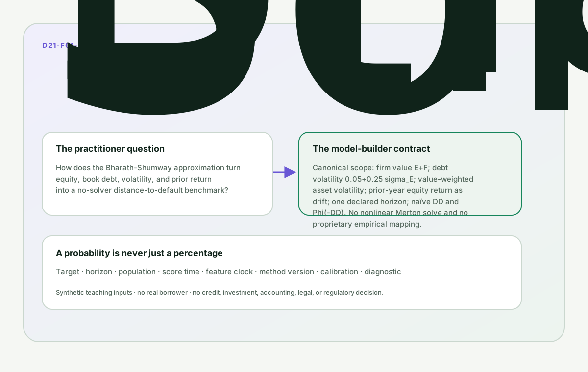
The opening view fixes the decision question and output context before presenting a percentage or score.
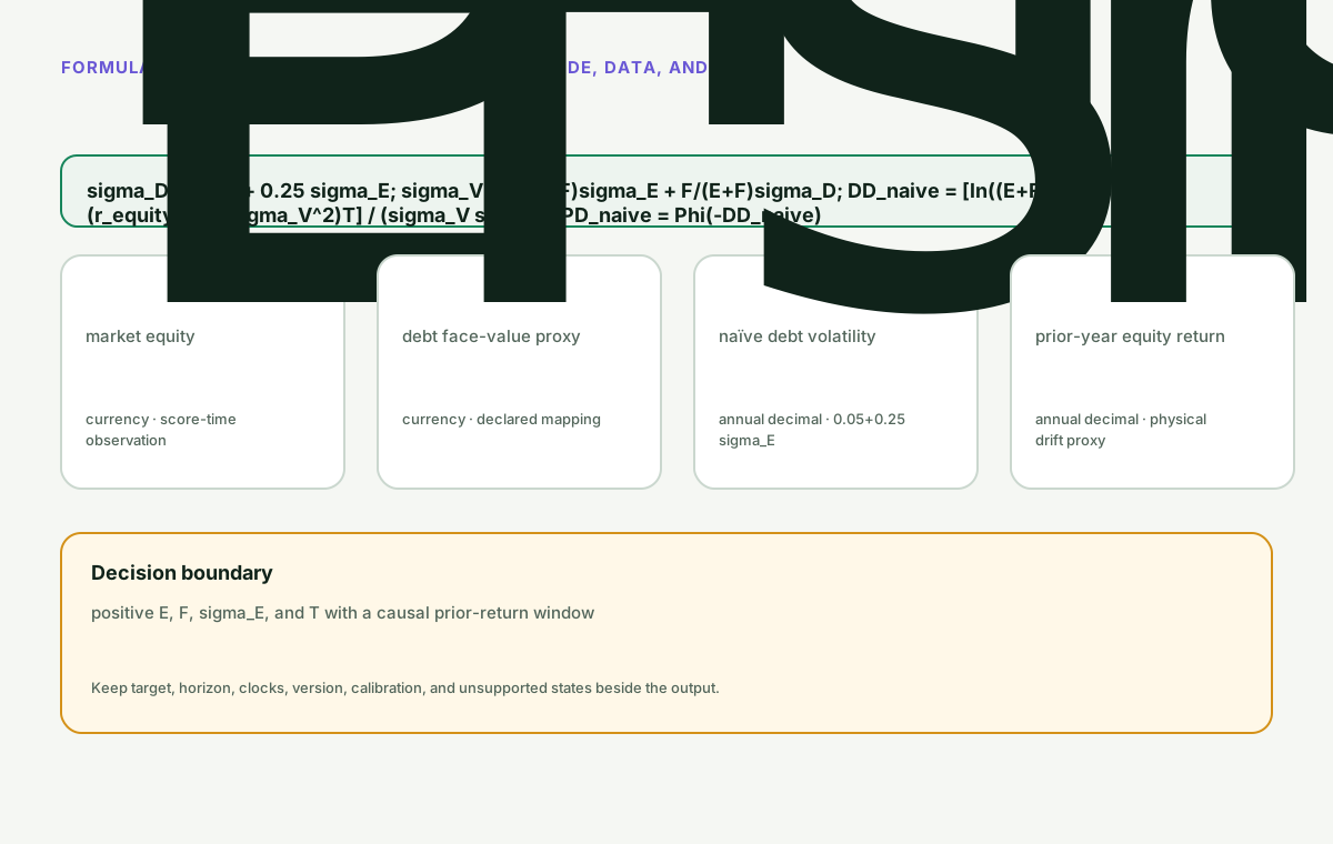
The formula view keeps units, selected conventions, and the material boundary beside the notation.
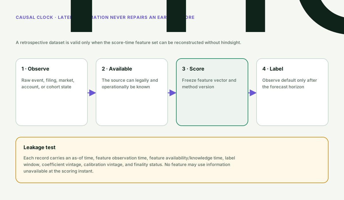
The clock view prevents a later filing, revised feature, market observation, or default label from leaking into the scoring state.
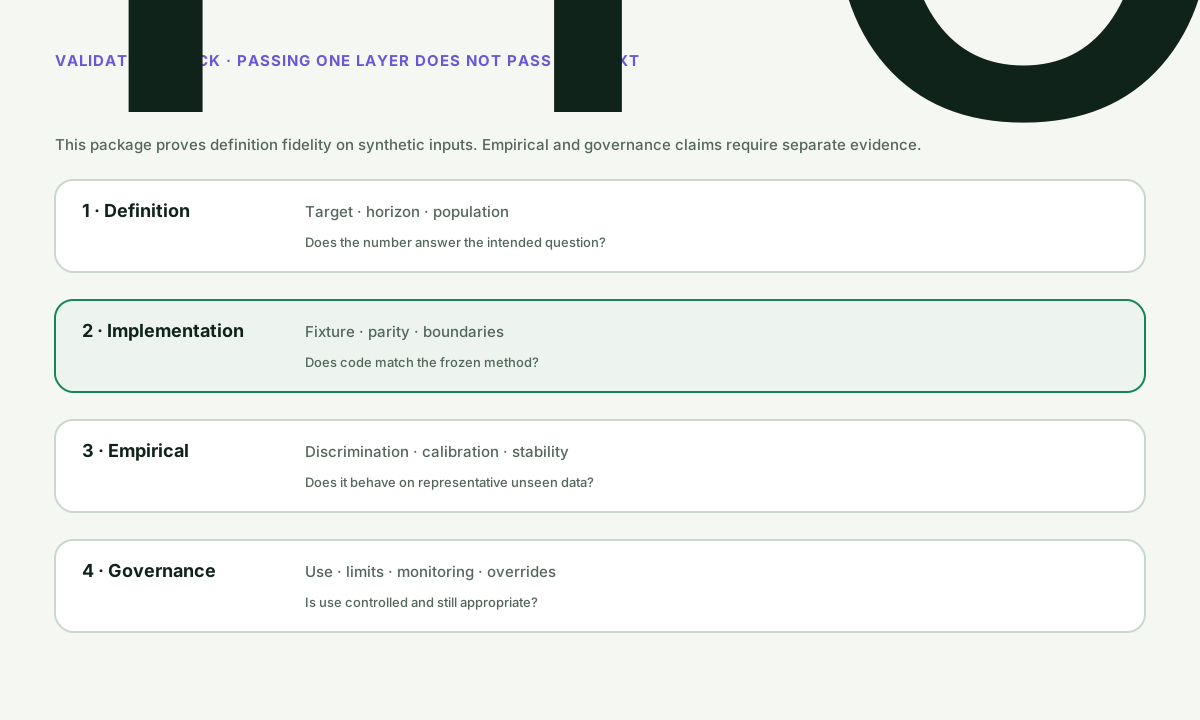
The validation view separates correct arithmetic from discrimination, calibration, stability, and governed use.
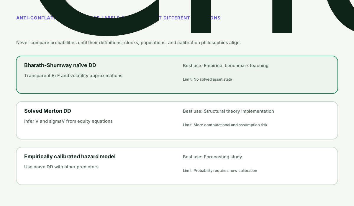
The comparison view shows why nearby methods cannot be substituted by output label alone.
Implementation walkthrough
The Python and TypeScript references begin with the same validation contract, reject malformed and unsupported state before calculation, preserve declared ordering and rounding policies, and return structured diagnostics rather than one context-free number.
The main implementation branches are:
- E, F, sigma_E, or T nonpositive — reject, because log and scale invalid.
- prior return window leaks forward — reject, because hindsight.
- compare with Merton — retain separate labels, because one solves V; one approximates V.
Neither reference silently fetches data, mutates caller-owned inputs outside the declared engine behavior, guesses hidden state, or substitutes a provider default. Shared JSON fixtures make value, null, state, and reason-code drift visible across languages.
Testing and validation
Definition tests compare every canonical field, reject malformed state, and exercise the material boundary. Family validation recomputes every playground state from the reference function. Independent arithmetic is recorded beside the fixture rather than inferred only from implementation output.
The audit must preserve these invariants:
- Input and feature lineage with availability time
- Coefficient and method version
- Intermediate score or structural state
- Probability and horizon
- Diagnostic state and reason code
Passing definition and parity checks proves that the implementation matches the selected contract. It does not prove production performance, universal applicability, or future empirical performance or borrower outcome.
Failure modes and misuse
- Definition fidelity and code parity do not establish discrimination, calibration, stability, fairness, approval suitability, regulatory compliance, or profitability.
- Rare-event labels, censoring, selection, survivorship, class imbalance, regime change, data revisions, and overrides can dominate apparent model precision.
- Outputs from different horizons, default definitions, populations, or calibration philosophies are not directly comparable.
- This educational package is not credit, investment, legal, accounting, or regulatory advice and must not be used to make decisions about real people or firms.
Debugging order
When a result looks surprising, inspect the state in this order:
- Confirm identifiers, scope, side, and decision clock.
- Confirm units, ordering, and point-in-time inputs.
- Confirm equality, rounding, null, and reset policies.
- Recalculate the invariant and declared scenario focus before changing code.
Evidence and historical boundary
Historical decision: not useful. A named borrower is not useful for the canonical mechanics: reproducible PD requires the exact default definition, sample selection, feature availability clock, coefficient vintage, calibration, overrides, use case, and permission to publish borrower data. Controlled synthetic records expose those choices without implying a real entity's creditworthiness.
The primary sources are Bharath-Shumway (2008), Merton (1974), 2026 interagency model-risk guidance. They support the source roles listed in the research ledger, not a redistributable historical observation, current calibration, regulatory approval, IFRS 9 compliance, borrower creditworthiness, causal interpretation, or investment value.
Summary and next topic
You can now calculate and distinguish the Bharath-Shumway naïve DD benchmark. The learning flow is: Campbell-Hilscher-Szilagyi Distress Probability → Bharath-Shumway Naive Distance-to-Default → Workout LGD. Carry the result forward only with its scope, clock, state, and evidence label.
Rendered from the canonical Mermaid sources linked by this article.
Bharath-Shumway Naive Distance-to-Default calculation flow
This flow identifies the selected calculation stages and the structured output.
Takeaway: The naïve benchmark is reproducible precisely because every shortcut is visible; it must never be mislabeled as solved Merton DD.
ReferencesPrimary sources and evidence notesExpand the source trail, evidence role, and limitations behind the engineering choices.
Expand the source trail, evidence role, and limitations behind the engineering choices.
S1 — Forecasting Default with the Merton Distance to Default Model
- Organization or authors: Sreedhar T. Bharath and Tyler Shumway
- Source type: Original peer-reviewed paper
- Publication or effective date: 2008-05-19
- Version: Review of Financial Studies 21(3), 1339-1369
- URL or DOI: https://doi.org/10.1093/rfs/hhn044
- Accessed: 2026-08-06
- Jurisdiction: United States listed-firm research sample
- Supports: The approximation is an empirical benchmark, not a solved Merton model or universal calibrated PD.
- Limitations: Applying it to another population requires point-in-time inputs, label alignment, and out-of-sample validation.
S2 — On the Pricing of Corporate Debt: The Risk Structure of Interest Rates
- Organization or authors: Robert C. Merton
- Source type: Original peer-reviewed paper
- Publication or effective date: 1974-05
- Version: Journal of Finance 29(2), 449-470
- URL or DOI: https://doi.org/10.1111/j.1540-6261.1974.tb03058.x
- Accessed: 2026-08-06
- Jurisdiction: Structural corporate-debt theory
- Supports: Equity can be represented as an option on firm assets under the paper's assumptions, connecting asset value, volatility, debt, and default at maturity.
- Limitations: The stylized assumptions do not identify a real firm's default point, physical drift, recovery, or empirical calibration.
S3 — Supervisory Guidance on Model Risk Management
- Organization or authors: OCC, Board of Governors of the Federal Reserve System, and FDIC
- Source type: Official interagency supervisory guidance
- Publication or effective date: 2026-04-17
- Version: SR 26-2 / interagency 2026 guidance
- URL or DOI: https://www.federalreserve.gov/frrs/guidance/supervisory-guidance-on-model-risk-management.htm
- Accessed: 2026-08-06
- Jurisdiction: United States banking organizations within stated scope
- Supports: Model use should reflect purpose, materiality, limitations, validation, monitoring, governance, and controls.
- Limitations: It is risk-based supervisory guidance, not a validation checklist that certifies these educational models.
Evidence boundary
The sources establish the exact rule, interface, protocol, or research context named above. They do not verify the repository-authored synthetic fixture, thresholds, empirical usefulness, execution probability, or profitability. Package-selected choices remain labeled as implementation choices wherever they are used.
Full dependency-light reference implementations in both supported languages.
/** Deterministic D21-F01 Probability of Default reference calculations. */

type RecordValue = Record<string, unknown>;

function numberValue(name: string, value: unknown): number {
  if (typeof value !== "number" || !Number.isFinite(value)) throw new Error(`${name} must be a finite number`);
  return value;
}

function positive(name: string, value: unknown): number {
  const parsed = numberValue(name, value);
  if (parsed <= 0) throw new Error(`${name} must be positive`);
  return parsed;
}

function probability(name: string, value: unknown, openInterval = false): number {
  const parsed = numberValue(name, value);
  const valid = openInterval ? parsed > 0 && parsed < 1 : parsed >= 0 && parsed <= 1;
  if (!valid) throw new Error(`${name} must be ${openInterval ? "strictly " : ""}between zero and one`);
  return parsed;
}

function vector(name: string, value: unknown, minimum = 1): number[] {
  if (!Array.isArray(value) || value.length < minimum) throw new Error(`${name} must contain at least ${minimum} finite numbers`);
  return value.map((item, index) => numberValue(`${name}[${index}]`, item));
}

function clean(value: number): number {
  const rounded = Math.round((value + Number.EPSILON) * 1e12) / 1e12;
  return Object.is(rounded, -0) ? 0 : rounded;
}

function sigmoid(score: number): number {
  if (score >= 0) { const tail = Math.exp(-score); return 1 / (1 + tail); }
  const head = Math.exp(score); return head / (1 + head);
}

// Abramowitz-Stegun 7.1.26; adequate for the package's 1e-7 cross-language tolerance.
function erf(value: number): number {
  const sign = value < 0 ? -1 : 1;
  const x = Math.abs(value);
  const t = 1 / (1 + 0.3275911 * x);
  const polynomial = ((((1.061405429 * t - 1.453152027) * t + 1.421413741) * t - 0.284496736) * t + 0.254829592) * t;
  const y = 1 - polynomial * Math.exp(-x * x);
  return sign * y;
}

function normalCdf(value: number): number { return 0.5 * (1 + erf(value / Math.sqrt(2))); }

function linearScore(intercept: unknown, coefficients: unknown, features: unknown): [number, number[]] {
  const constant = numberValue("intercept", intercept);
  const beta = vector("coefficients", coefficients);
  const x = vector("features", features);
  if (beta.length !== x.length) throw new Error("coefficients and features must have equal length");
  const contributions = beta.map((item, index) => clean(item * x[index]));
  return [clean(constant + contributions.reduce((sum, item) => sum + item, 0)), contributions];
}

export function logisticPdModel(intercept: unknown, coefficients: unknown, features: unknown, alert_threshold: unknown): RecordValue {
  const [score, contributions] = linearScore(intercept, coefficients, features);
  const threshold = probability("alert_threshold", alert_threshold, true);
  const pd = sigmoid(score);
  return {
    linear_score: clean(score), feature_contributions: contributions,
    probability_of_default: clean(pd), survival_probability: clean(1 - pd),
    odds_of_default: clean(pd / (1 - pd)), alert_threshold: clean(threshold),
    state: pd >= threshold ? "at-or-above-alert" : "below-alert",
    reason: "supplied-logit-score-transformed",
  };
}

export function probitPdModel(intercept: unknown, coefficients: unknown, features: unknown, alert_threshold: unknown): RecordValue {
  const [score, contributions] = linearScore(intercept, coefficients, features);
  const threshold = probability("alert_threshold", alert_threshold, true);
  const pd = normalCdf(score);
  return {
    latent_score: clean(score), feature_contributions: contributions,
    probability_of_default: clean(pd), survival_probability: clean(1 - pd),
    alert_threshold: clean(threshold), state: pd >= threshold ? "at-or-above-alert" : "below-alert",
    reason: "supplied-probit-score-transformed",
  };
}

export function throughTheCyclePd(annual_obligors: unknown, annual_defaults: unknown, current_year_index: unknown, minimum_years: unknown): RecordValue {
  const obligors = vector("annual_obligors", annual_obligors, 2);
  const defaults = vector("annual_defaults", annual_defaults, 2);
  if (obligors.length !== defaults.length) throw new Error("annual_obligors and annual_defaults must have equal length");
  const minimum = positive("minimum_years", minimum_years);
  if (!Number.isInteger(minimum) || obligors.length < minimum) throw new Error("minimum_years must be an integer no greater than the history length");
  const index = numberValue("current_year_index", current_year_index);
  if (!Number.isInteger(index) || index < 0 || index >= obligors.length) throw new Error("current_year_index must select an observed year");
  const rates = obligors.map((population, year) => {
    const count = defaults[year];
    if (population <= 0) throw new Error(`annual_obligors[${year}] must be positive`);
    if (!Number.isInteger(count) || count < 0 || count > population) throw new Error(`annual_defaults[${year}] must be an integer from zero to obligors`);
    return count / population;
  });
  const ttc = rates.reduce((sum, item) => sum + item, 0) / rates.length;
  const pooled = defaults.reduce((sum, item) => sum + item, 0) / obligors.reduce((sum, item) => sum + item, 0);
  const current = rates[index];
  return {
    annual_default_rates: rates.map(clean), through_the_cycle_pd: clean(ttc), pooled_default_rate: clean(pooled),
    current_observed_default_rate: clean(current), cycle_gap: clean(current - ttc), observation_years: rates.length,
    state: current > ttc ? "current-above-long-run" : current < ttc ? "current-below-long-run" : "current-equals-long-run",
    reason: "simple-average-of-annual-one-year-rates",
  };
}

export function pointInTimePd(through_the_cycle_pd_value: unknown, borrower_log_odds_shift: unknown, macro_factor_z: unknown, macro_sensitivity: unknown, alert_threshold: unknown): RecordValue {
  const ttc = probability("through_the_cycle_pd", through_the_cycle_pd_value, true);
  const borrowerShift = numberValue("borrower_log_odds_shift", borrower_log_odds_shift);
  const macro = numberValue("macro_factor_z", macro_factor_z);
  const sensitivity = numberValue("macro_sensitivity", macro_sensitivity);
  if (sensitivity < 0) throw new Error("macro_sensitivity must be nonnegative under this package convention");
  const threshold = probability("alert_threshold", alert_threshold, true);
  const baselineLogOdds = Math.log(ttc / (1 - ttc));
  const macroShift = sensitivity * macro;
  const pd = sigmoid(baselineLogOdds + borrowerShift + macroShift);
  return {
    through_the_cycle_pd: clean(ttc), baseline_log_odds: clean(baselineLogOdds), borrower_log_odds_shift: clean(borrowerShift),
    macro_log_odds_shift: clean(macroShift), point_in_time_pd: clean(pd), cycle_uplift: clean(pd - ttc),
    alert_threshold: clean(threshold), state: pd >= threshold ? "at-or-above-alert" : "below-alert",
    reason: "declared-log-odds-overlay-not-universal-ifrs-or-regulatory-formula",
  };
}

function mertonTerms(asset: number, sigma: number, debt: number, rate: number, horizon: number): [number, number] {
  const scale = sigma * Math.sqrt(horizon);
  const d1 = (Math.log(asset / debt) + (rate + 0.5 * sigma * sigma) * horizon) / scale;
  return [d1, d1 - scale];
}

export function mertonDistanceToDefault(equity_value: unknown, equity_volatility: unknown, debt_face_value: unknown, risk_free_rate: unknown, asset_drift: unknown, horizon_years: unknown, tolerance: unknown, max_iterations: unknown): RecordValue {
  const equity = positive("equity_value", equity_value), sigmaEquity = positive("equity_volatility", equity_volatility);
  const debt = positive("debt_face_value", debt_face_value), rate = numberValue("risk_free_rate", risk_free_rate);
  const drift = numberValue("asset_drift", asset_drift), horizon = positive("horizon_years", horizon_years);
  const tol = positive("tolerance", tolerance), limit = positive("max_iterations", max_iterations);
  if (!Number.isInteger(limit) || limit > 10000) throw new Error("max_iterations must be an integer no greater than 10000");
  let asset = equity + debt * Math.exp(-rate * horizon), sigmaAsset = Math.min(3, Math.max(1e-6, sigmaEquity * equity / asset));
  let residual = Number.POSITIVE_INFINITY, converged = false, iterations = 0;
  for (iterations = 1; iterations <= limit; iterations += 1) {
    const [d1, d2] = mertonTerms(asset, sigmaAsset, debt, rate, horizon), n1 = normalCdf(d1), n2 = normalCdf(d2);
    if (n1 <= 1e-14) break;
    const nextAsset = (equity + debt * Math.exp(-rate * horizon) * n2) / n1;
    const nextSigma = sigmaEquity * equity / (nextAsset * n1);
    residual = Math.max(Math.abs(nextAsset - asset) / Math.max(asset, 1), Math.abs(nextSigma - sigmaAsset));
    asset = nextAsset; sigmaAsset = nextSigma;
    if (residual <= tol) { converged = true; break; }
  }
  if (!converged) return { asset_value: null, asset_volatility: null, distance_to_default: null, physical_default_probability: null, risk_neutral_default_probability: null, iterations: Math.min(iterations, limit), residual: Number.isFinite(residual) ? clean(residual) : null, state: "not-converged", reason: "merton-equity-system-did-not-converge" };
  const [, d2] = mertonTerms(asset, sigmaAsset, debt, rate, horizon);
  const dd = (Math.log(asset / debt) + (drift - 0.5 * sigmaAsset * sigmaAsset) * horizon) / (sigmaAsset * Math.sqrt(horizon));
  return { asset_value: clean(asset), asset_volatility: clean(sigmaAsset), distance_to_default: clean(dd), physical_default_probability: clean(normalCdf(-dd)), risk_neutral_default_probability: clean(normalCdf(-d2)), iterations, residual: clean(residual), state: "converged", reason: "merton-equity-system-solved" };
}

export function campbellHilscherSzilagyiDistressProbability(nimtaavg: unknown, tlmta: unknown, exretavg: unknown, sigma: unknown, rsize: unknown, cashmta: unknown, market_to_book: unknown, log_price: unknown): RecordValue {
  const values: Record<string, number> = { nimtaavg: numberValue("nimtaavg", nimtaavg), tlmta: numberValue("tlmta", tlmta), exretavg: numberValue("exretavg", exretavg), sigma: numberValue("sigma", sigma), rsize: numberValue("rsize", rsize), cashmta: numberValue("cashmta", cashmta), market_to_book: numberValue("market_to_book", market_to_book), log_price: numberValue("log_price", log_price) };
  if (values.sigma < 0 || values.tlmta < 0 || values.cashmta < 0) throw new Error("sigma, tlmta, and cashmta must be nonnegative");
  const beta: Record<string, number> = { nimtaavg: -20.264, tlmta: 1.416, exretavg: -7.129, sigma: 1.411, rsize: -0.045, cashmta: -2.132, market_to_book: 0.075, log_price: -0.058 };
  const contributions: Record<string, number> = {};
  Object.keys(values).forEach(key => { contributions[key] = clean(values[key] * beta[key]); });
  const score = -9.164 + Object.values(contributions).reduce((sum, item) => sum + item, 0);
  return { published_intercept: -9.164, score_contributions: contributions, failure_log_odds: clean(score), distress_probability: clean(sigmoid(score)), state: "published-score-replication", reason: "chs-table-4-twelve-month-lag-coefficients" };
}

export function bharathShumwayNaiveDistanceToDefault(equity_value: unknown, debt_face_value: unknown, equity_volatility: unknown, prior_year_equity_return: unknown, horizon_years: unknown): RecordValue {
  const equity = positive("equity_value", equity_value), debt = positive("debt_face_value", debt_face_value);
  const sigmaEquity = positive("equity_volatility", equity_volatility), drift = numberValue("prior_year_equity_return", prior_year_equity_return), horizon = positive("horizon_years", horizon_years);
  const firm = equity + debt, sigmaDebt = 0.05 + 0.25 * sigmaEquity;
  const sigmaAsset = (equity / firm) * sigmaEquity + (debt / firm) * sigmaDebt;
  const dd = (Math.log(firm / debt) + (drift - 0.5 * sigmaAsset * sigmaAsset) * horizon) / (sigmaAsset * Math.sqrt(horizon));
  return { naive_firm_value: clean(firm), naive_debt_volatility: clean(sigmaDebt), naive_asset_volatility: clean(sigmaAsset), naive_distance_to_default: clean(dd), naive_default_probability: clean(normalCdf(-dd)), state: "calculated", reason: "bharath-shumway-naive-approximation" };
}

export function calculate(topicId: string, inputs: RecordValue): RecordValue {
  if (!inputs || typeof inputs !== "object" || Array.isArray(inputs)) throw new Error("inputs must be an object");
  switch (topicId) {
    case "D21-F01-A01": return logisticPdModel(inputs.intercept, inputs.coefficients, inputs.features, inputs.alert_threshold);
    case "D21-F01-A02": return probitPdModel(inputs.intercept, inputs.coefficients, inputs.features, inputs.alert_threshold);
    case "D21-F01-A03": return throughTheCyclePd(inputs.annual_obligors, inputs.annual_defaults, inputs.current_year_index, inputs.minimum_years);
    case "D21-F01-A04": return pointInTimePd(inputs.through_the_cycle_pd_value, inputs.borrower_log_odds_shift, inputs.macro_factor_z, inputs.macro_sensitivity, inputs.alert_threshold);
    case "D21-F01-A05": return mertonDistanceToDefault(inputs.equity_value, inputs.equity_volatility, inputs.debt_face_value, inputs.risk_free_rate, inputs.asset_drift, inputs.horizon_years, inputs.tolerance, inputs.max_iterations);
    case "D21-F01-A06": return campbellHilscherSzilagyiDistressProbability(inputs.nimtaavg, inputs.tlmta, inputs.exretavg, inputs.sigma, inputs.rsize, inputs.cashmta, inputs.market_to_book, inputs.log_price);
    case "D21-F01-A07": return bharathShumwayNaiveDistanceToDefault(inputs.equity_value, inputs.debt_face_value, inputs.equity_volatility, inputs.prior_year_equity_return, inputs.horizon_years);
    default: throw new Error(`unsupported topic_id: ${topicId}`);
  }
}
The embedded lab now expands to its full document height, keeping the article as the only scroll surface.