Five-Number Summary and Box Plot

Synthetic teaching data · Type-7 quantiles where applicable · Python and TypeScript verification

Start with the human question

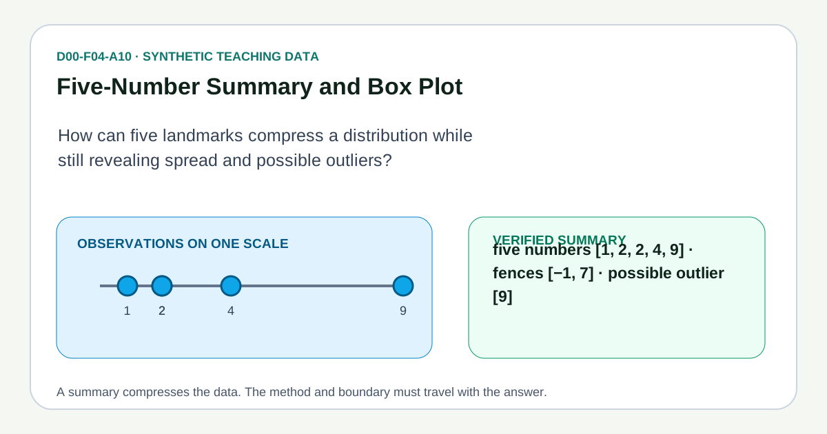
How can five landmarks compress a distribution while still revealing spread and possible outliers? That question is more important than the formula. A statistic is useful only when its mechanical definition matches the thing a reader is trying to learn.

The five-number summary is minimum, Q1, median, Q3, and maximum. A box plot draws Q1 to Q3 as a box, marks the median, and uses an explicit whisker and outlier convention. It compresses a list into a smaller description. Compression is helpful, but it always loses information. This tutorial repeatedly shows both the preserved signal and the discarded detail so that a beginner does not mistake a neat number for a complete explanation.

One-minute answer

The frozen rule is IQR = Q3−Q1; inner fences = Q1−1.5IQR and Q3+1.5IQR; whiskers stop at extreme observations within fences. On the canonical synthetic values, the verified answer is five numbers [1, 2, 2, 4, 9] · fences [−1, 7] · possible outlier [9]. Keep the input count, method convention, and data-cleaning policy next to that answer.

See the data before summarizing it

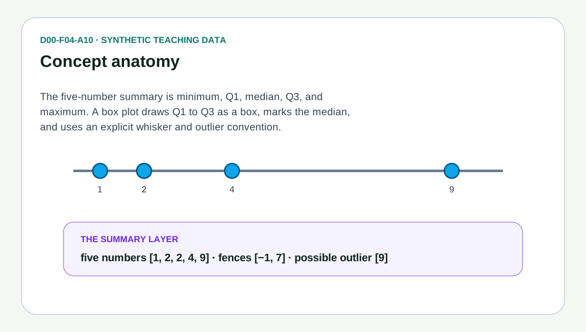
Each mark in the picture is an observation. The emphasized layer is the summary produced by this topic. Notice that several different raw datasets can produce the same summary. That is not a bug; it is the price of compression. It is why a responsible report pairs a compact statistic with a distribution view or a clearly scoped statement.

The teaching fixture uses [1, 2, 2, 4, 9]. It is deliberately small enough to sort on paper and deliberately uneven enough to expose an endpoint, a tie, and a gap. The values are synthetic. They make no claim about a real asset, provider, or period.

Build the answer one line at a time

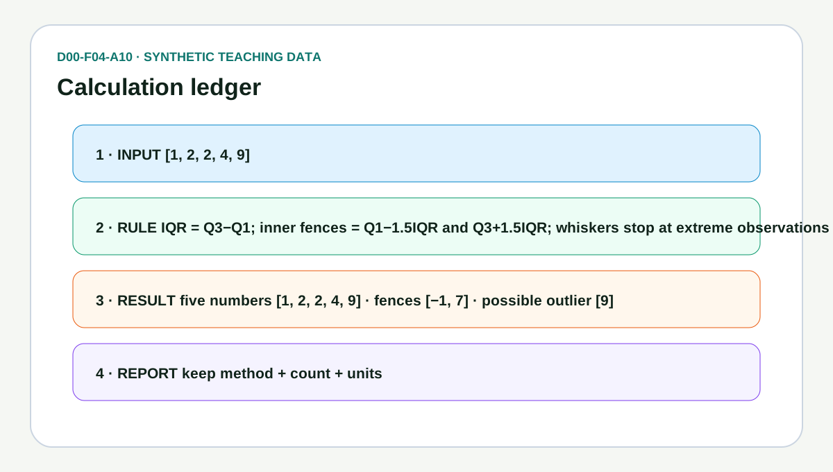
Type-7 landmarks for [1, 2, 2, 4, 9] are [1, 2, 2, 4, 9]. IQR is 2, inner fences are −1 and 7, so 9 is plotted as a possible outlier and the upper whisker stops at 4. The ledger uses full-precision arithmetic. Display rounding occurs only after the algorithm returns its result, so a rounded intermediate value cannot leak into the next step.

Try the same work manually:

1. Write the supplied values and count them.
2. Sort a copy when the method depends on order; do not mutate the original record silently.
3. Apply the named rule exactly, including its denominator, tie policy, interpolation method, or bin boundary.
4. Keep enough digits to verify the result.
5. Explain the answer in a sentence that includes its boundary.

If your manual result disagrees with the fixture, stop before interpretation. Check the input, the method, and the policy—not only the arithmetic.

The decision contract

The implementation accepts a nonempty array of finite numbers. Topic-specific fields such as weights, trim proportion, or bin count are explicit. It rejects an undefined state instead of converting it to zero. That strictness is educational: “not computable from this input” is an important result.

The package also freezes type-7 linear interpolation for quartiles and medians where interpolation is needed. Percentile methods can differ, particularly in small samples. Naming the method makes Python, TypeScript, an article, and a future data pipeline reproduce the same answer.

What can go wrong?

A flagged point is not automatically an error. It is a prompt to investigate context, measurement, and distribution assumptions.

Not every box plot draws whiskers at the minimum and maximum. State whether whiskers use data endpoints, fences, or another rule.

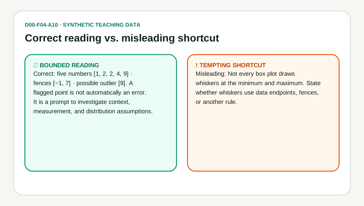
The right-hand side of the illustration is tempting because it sounds decisive. The left-hand side is more useful because it states exactly what was calculated and what remains unknown. This habit—claiming only what the method supports—is foundational to every later financial model.

Compare nearby tools

A09 shows more shape detail. A box plot is compact and excellent for comparing several groups on the same scale.

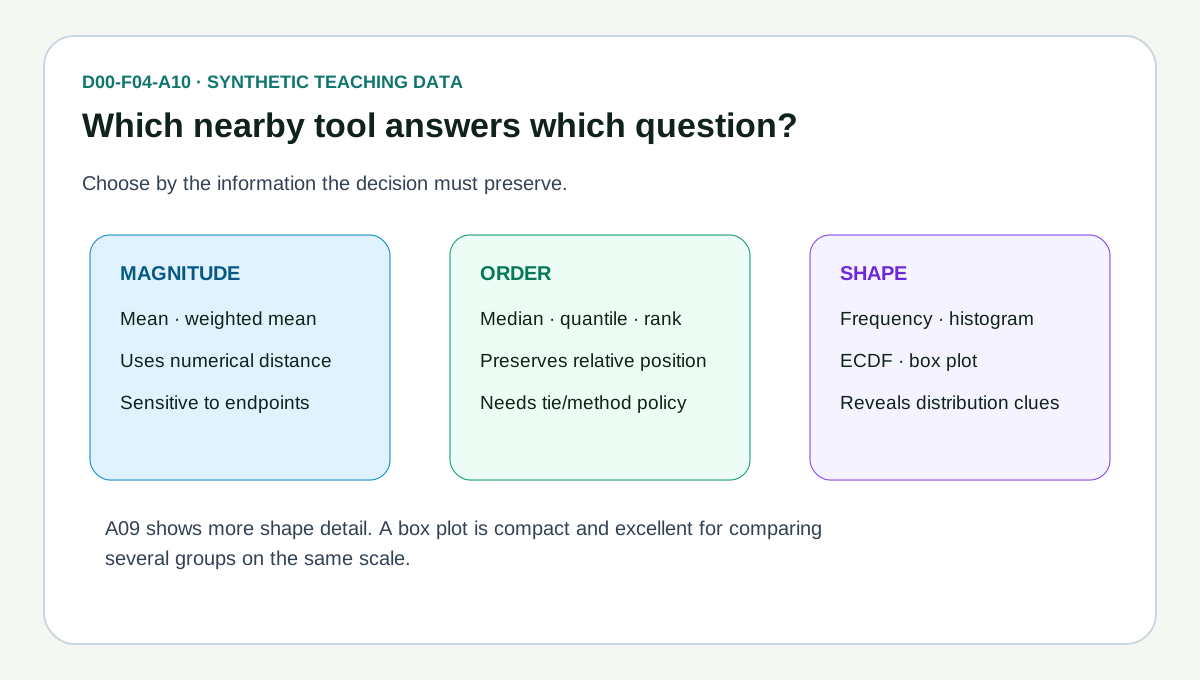
No summary wins every comparison. Magnitude-sensitive measures notice changes that rank-based measures can resist. Compact plots support group comparison but hide detail that a histogram or ECDF retains. The correct question is not “Which statistic is best?” It is “Which information must this decision preserve?”

Five scenarios that create intuition

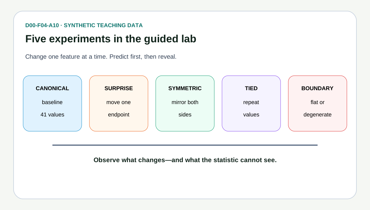
The guided lab supplies five datasets with 41 observations each:

• Canonical: a stable, mildly skewed baseline.
• Surprise value: one endpoint moves while the other 40 observations remain fixed.
• Symmetric: changes on one side are mirrored on the other.
• Tied or flat: repeated values expose mode and rank policies.
• Boundary: constant or nearly constant data reveals degenerate ranges, bins, quartiles, and outlier rules.

Before revealing a new state, predict which output should change. Prediction converts a moving picture into an experiment. The audit panel then explains what moved, what stayed fixed, and why.

A financial-data example without a market claim

Imagine the values are five validated transaction costs in basis points. The arithmetic is identical, but the interpretation now needs units, sampling rules, timestamps, venue scope, and a missing-value policy. A summary of costs is not evidence that an execution strategy caused those costs, and it is not a forecast of the next trade.

That distinction is why the package keeps the example synthetic. The lesson transfers to prices, returns, spreads, volumes, durations, and fundamental ratios only after those data contracts are defined.

Implementation notes

The narrow Python and TypeScript topic facades delegate arithmetic to the reviewed shared D00 engine. Both consume the same JSON fixture. The implementation returns unrounded values and makes undefined denominators or empty inputs visible through errors. This package does not invent a separate browser-only definition: the playground labels its method and mirrors the canonical contract.

Pseudocode

validate the required finite inputs
copy the observations
apply the frozen five-number summary and box plot rule
return the numerical result plus useful audit fields
never silently change the method or missing-value policy

Checklist for a trustworthy explanation

• Did I show the observation count and units?
• Did I name any weighting, tie, quantile, trimming, bin, or whisker convention?
• Did I keep synthetic and historical evidence clearly labeled?
• Did I show at least one dataset where the statistic gives an incomplete picture?
• Did I avoid treating a possible outlier as an automatic error?
• Can another implementation reproduce the full-precision output?
• Does my sentence claim only what this summary actually measures?

Final takeaway

The five-number summary is minimum, Q1, median, Q3, and maximum. A box plot draws Q1 to Q3 as a box, marks the median, and uses an explicit whisker and outlier convention. For the worked case, five numbers [1, 2, 2, 4, 9] · fences [−1, 7] · possible outlier [9]. The number becomes trustworthy only when the input, method, and limitation travel with it.

Open the guided lab next and move the surprise value. Watch which summaries react immediately and which barely move. That contrast is the fastest route from memorizing a formula to understanding it.

Previous: D00-F04-A09 · Next: family complete