
 By Islam Baraka
Calculate the return implied by supplied factor exposures and premia, and identify the assumption behind any apparent pricing gap. The useful result is not just a scalar. You should be able to trace it back to eligible observations, explain which convention produced it and recognize when the calculation should stop.
This tutorial builds A finite-factor expected-return calculator with supplied loadings and premia. It does not estimate latent factors or declare an executable arbitrage. You will calculate a small example, run matching Python and TypeScript implementations, inspect a controlled synthetic case and change one assumption in a guided lab. No historical market performance is claimed.
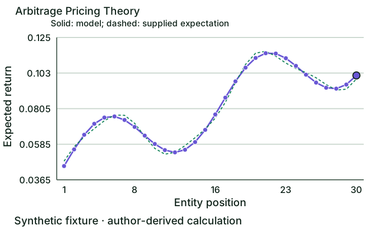
The chart shows the canonical fixture. Read the axis units before comparing values: a return, a score, a weight and a statistical diagnostic are different objects. Its numerical source is the same fixture used by the executable examples. Open the full-size chart when you need to inspect small labels.
Start with the question, then the mechanism
Each factor is a priced unit of exposure. Multiplying exposure by its premium produces a contribution in return units, and adding these contributions to the risk-free base yields the model expectation. Scale a factor by ten and its loading must scale by one tenth; the contribution should stay unchanged. This simple invariance is an important test because an apparently sophisticated factor model can otherwise change merely because someone switched a factor from decimal to percentage units.
Use a single currency and horizon; compare like-for-like expectations without fitting premia to erase the same discrepancies.
From fitted exposure to a pricing claim
There are three different questions in asset pricing. A time-series fit asks how an asset moved with supplied factors. A pricing restriction asks what its expected return should be. A trading decision asks whether a feasible position offers an attractive return after costs and uncertainty. The same coefficient cannot answer all three questions. Keep the expected-return assumption outside the realized-return regression until you have evidence that connects them.
For regression topics, arrange observations in chronological rows, include an intercept, and express every return in decimal units at the same frequency. Subtract the same-period risk-free return once from the asset. Do not subtract it again from a self-financing spread. The factor order is part of the API: a correct vector multiplied by mislabeled columns is a wrong model. Estimate all included columns jointly; one regression per factor does not estimate partial exposures.
The implementation uses reorthogonalized, column-scaled QR to solve least squares. This avoids explicitly forming the normal equations for the coefficient estimate. A column that becomes numerically dependent on earlier columns causes a rejection. Bartlett HAC covariance describes sampling uncertainty under appropriate weak-dependence conditions; it does not repair endogeneity, structural breaks, a mismatched benchmark, or an unrepresentative sample. The intercept remains a per-period return, not an automatically annualized alpha.
Before presenting results, inspect the residual series and fitted-versus-observed plot. Compare an economically motivated competing specification using the same dates. A smaller in-sample residual is expected when adding regressors; it is not by itself a reason to select the larger model. Out-of-sample evidence, model stability and the intended use determine whether the extra exposure estimates are helpful. The APT calculator is deliberately different: it accepts premia as assumptions rather than estimating them from this regression machinery.
Freeze the definition
b is a dimensionless factor exposure matrix; lambda is a vector of same-horizon risk premia; r_f and mu are same-horizon expected simple returns; g is a model discrepancy.
The sources establish the method's research context; the stated variant fixes the implementation choices for this package. See Ross (1976), The Arbitrage Theory of Capital Asset Pricing. Where a teaching convention differs from a published portfolio or test, it is labeled explicitly rather than borrowing the published method's empirical conclusions.
Work a small example before running the code
With r_f=0.02, exposures (1.2,-0.5) and premia (0.05,0.02), implied expected return is 0.02+1.2×0.05-0.5×0.02=0.07. A supplied expectation of 0.08 creates a model gap of 0.01, or one percentage point. It does not identify a costless, riskless trade.
The machine-readable hand check is saved separately from the larger chart fixture. It asserts implied_returns against [0.07]. Some hand checks use a different small input from the prose example to test the same invariant from another direction. For a model with several regressors, a one-row attribution example cannot estimate the loadings; the multi-period executable fixture supplies the necessary observations.
To audit the arithmetic, carry full precision through intermediate values and round only for display. Ask whether the result's unit is consistent with the formula. Then consider a limiting case: does the method return an explicit rejection or undefined result when its denominator or identifying variation disappears?
Prepare data without borrowing from the future
| Input | Type | Meaning |
|---|---|---|
| exposures | number[][] | One row per asset and one column per factor. |
| premia | number[] | Same-horizon expected excess returns. |
| risk_free | number | Expected risk-free simple return. |
| expected_returns | number[] | Independently supplied expected total returns for discrepancy reporting. |
All calls also require formation_at, inputs_available_at and as_of as real ISO calendar dates. Inputs must be available by formation; formation cannot exceed the evaluation cutoff. Evaluation topics additionally require outcome start, end and availability dates. These envelope checks reject impossible chronology but cannot certify the provenance of individual rows. Your adapter must verify IDs, timestamps, frequency, currency, total-return adjustments, release dates and source vintages before building the arrays.
Missing, nonfinite, boolean or string-valued numbers are not silently repaired. The complete-case contract is intentional: changing eligibility changes the quantity being measured. Preserve the rejected records and the reason in a data-quality report, then choose a documented repair or a different model. Do not turn an undefined quantity into zero to make a chart look complete.
Follow the execution path
- Declare factor units. Use a single currency and horizon; compare like-for-like expectations without fitting premia to erase the same discrepancies.
- Read the exposures. Retain the inputs and the intermediate quantities; alignment is part of correctness.
- Price each factor leg. Calculate at full precision using the declared variant, not a convenient substitute.
- Add the risk-free base. Check the method’s invariant and preserve undefined outcomes separately from numeric zero.
- Bound the discrepancy. A positive model gap is not an arbitrage certificate. Factor selection, estimation error, residual risk, funding and portfolio feasibility remain separate.
Run the reference implementation
From the downloaded topic directory:
python examples/run.py
python -m unittest discover -s tests -p "test_*.py"
npx tsc -p implementations/typescript/tsconfig.json
node tests/test-typescript.mjs
The Python calculation has no third-party runtime dependency. TypeScript needs a compiler and an ES2022-capable JavaScript runtime. The public call accepts one JSON-shaped input and returns a discriminated success or error object. A minimal Python integration is:
from pathlib import Path
import importlib.util, json

root = Path.cwd()  # Run from this topic directory.
spec = importlib.util.spec_from_file_location("topic", root / "implementations/python/algorithm.py")
module = importlib.util.module_from_spec(spec)
spec.loader.exec_module(module)
data = json.loads((root / "datasets/canonical-input.json").read_text())
result = module.compute(data)
if result["status"] != "ok":
    raise ValueError(result["code"])
print(result["primary"])
After compilation, the equivalent TypeScript module can be used from JavaScript:
import { readFileSync } from 'node:fs';
import { compute } from './implementations/typescript/dist/algorithm.js';
const input = JSON.parse(readFileSync('./datasets/canonical-input.json', 'utf8'));
const result = compute(input);
if (result.status !== 'ok') throw new Error(result.code);
console.log(result.primary);
The canonical primary display is 0.045. More informative output fields include:
| Field | Canonical value / first values |
|---|---|
| contributions | [[0.025, 0], [0.0275, 0.00778836685], [0.03, 0.0143471218], [0.0325, 0.0186407817], [0.035, 0.0199914721], [0.0375, 0.0181859485], …] |
| implied_returns | [0.045, 0.0552883668, 0.0643471218, 0.0711407817, 0.0749914721, 0.0756859485, …] |
| gaps | [0.003, 0.00162090692, -0.00124844051, -0.00296997749, -0.00196093086, 0.000850986556, …] |
Inspect the complete returned object rather than reducing every use case to primary. That field is a playground convenience; the named intermediate and result fields preserve the method's meaning. Both languages use the same defaults and reason codes and do not mutate the input. Package tests compare the whole output tree, while independent mathematical checks avoid treating one implementation as the sole authority for the other.
Use the playground as an experiment
Open the topic's Playground tab or the self-contained guided lab. It starts from a meaningful canonical preview. Choose a scenario, predict the result, use Step to follow the calculation, and explain the evidence before pressing Play. Back and Reset let you revisit exactly the same state. Reduced-motion mode advances one deliberate step instead of running a timed sequence.
The main control is Second factor premium, ranging from -0.03 to 0.06 with default 0.02. The comparison scenario is Second-factor units multiplied by ten. Rescaling exposure and premium inversely must preserve every implied return. Every change recomputes the result through the validated TypeScript kernel; it does not select a prerecorded result.
The deliberate failure scenario, Missing factor premium, should return LENGTH_MISMATCH. First explain which assumption failed. Then return to the canonical case and identify the information that makes the calculation possible. This rejection is part of the lesson: it prevents an invalid model from producing a plausible-looking number.
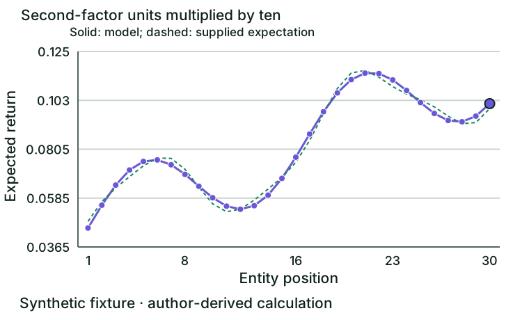
This second chart uses the comparison scenario at the default parameter. The caption and diagnostics in the lab explain what changes and what remains invariant. Identical output can be the correct outcome of an invariance experiment; do not mistake it for a broken control.
Avoid these interpretation failures
- Exposures and premia must use compatible factor normalization.
- A fitted expected-return gap can disappear out of sample.
- A zero-cost portfolio can still carry residual risk and leverage constraints.
A positive model gap is not an arbitrage certificate. Factor selection, estimation error, residual risk, funding and portfolio feasibility remain separate.
Check your understanding
Predict: What must change if an exposure column is expressed in units ten times larger?
Explain: Its premium must be divided by ten to preserve the implied return. Changing only one side changes the economic assumption.
Investigate: Run the canonical case, the comparison and the deliberate rejection. Save the input, output and one sentence explaining each difference. Identify a field whose unit could be confused with another field, and describe the consequence of that confusion.
Transfer: Before substituting real data, write the upstream eligibility and alignment rules. Name the source vintage, decision time and missing-value policy. Then identify one out-of-sample or data-quality check needed for your intended use. A successful synthetic calculation is a correctness demonstration, not evidence that the market rewards the signal.
What this package does and does not establish
The implementation makes the declared formula reproducible, exposes intermediates and rejects known invalid inputs. The sources motivate the method. The synthetic fixture lets you control one mechanism at a time. A named historical case remains deferred until its source observations and decision-time provenance can be archived; no invented returns are presented as real history.
Production use needs dataset-specific validation, monitored numerical limits, error logging, independent review and an execution or inference design appropriate to the application. See the source-package data contract and reference ledger for the full boundary. Educational material is not a recommendation to buy, sell or allocate capital.
Sources and further reading
- Ross (1976), The Arbitrage Theory of Capital Asset Pricing. Linear pricing restriction under no-arbitrage assumptions; does not identify a unique empirical factor set.
Choosing the method and continuing the lesson
This lesson is for analysts and developers who can work with aligned numerical arrays, means and return units. Regression and statistical-test topics also assume familiarity with residuals and sampling uncertainty; review the linked prerequisite before interpreting an inferential result.
| Decision | Declared approach | Neighbor or alternative |
|---|---|---|
| APT versus CAPM | Allows a specified collection of systematic factors under no-arbitrage reasoning. | CAPM is an equilibrium restriction based on the market portfolio. |
| Expected premium versus realized factor return | Used to price an expectation. | Used to attribute a realized period outcome. |
Use the declared approach when its input and interpretation match your research question. If you choose the alternative, freeze a new convention and rerun the examples; changing a label is not enough to change the calculation.
Related concepts
Excess return, Total return. For any use with observed market data, keep the point-in-time dataset boundary explicit.
Learning connections
- Prerequisite: CAPM Beta. Establish the inputs or mathematical distinction used here.
- Comparison: CAPM Beta. Compare its question and output units before substituting it for this method.
- Continue with: Value Factor Score. Carry the same formation clock and declared units into the next calculation.
Rendered from the canonical Mermaid sources linked by this article.
Calculation flow
ReferencesPrimary sources and evidence notesExpand the source trail, evidence role, and limitations behind the engineering choices.
Expand the source trail, evidence role, and limitations behind the engineering choices.
Ross (1976), The Arbitrage Theory of Capital Asset Pricing
- Source: Ross (1976), The Arbitrage Theory of Capital Asset Pricing
- Version / date: 1976
- Accessed: 2026-09-22
- Supports: Linear pricing restriction under no-arbitrage assumptions; does not identify a unique empirical factor set.
- Limitations: methodological context only; no claim that the source validates this synthetic sample or every educational convention.
- Reuse: cited, not copied. No source dataset is redistributed.
Evidence boundaries
The formulas are operationalized in the canonical README with explicit package conventions. Original synthetic fixtures isolate mechanisms and are not a historical performance claim. External source access can be restricted; the MacKinlay archive is a bibliographic reference, not a claim that its full text was retrieved during this build.
Historical case decision: deferred. A named empirical case would require a separately archived point-in-time universe, source vintage and outcome design. A synthetic control is used here to demonstrate pricing plane without attributing invented observations to a market. This limits empirical coverage; it does not change the mathematical contract.
When using live data, archive the retrieval date, provider query, license, currency, frequency, adjustment basis and transformation log. Do not imply that the primary authors endorsed this educational implementation.
Full dependency-light reference implementations in both supported languages.
/** D17 reference algorithms. JSON boundary validation is deliberate and shared.
 * Arrays are copied before sorting; callers' inputs are never mutated.
 * QR solves least squares without forming normal equations.
 */
type Data = Record<string, any>;
type Result = Record<string, any>;
class ContractError extends Error {
}
const fail = (code: string): never => { throw new ContractError(code); };
const num = (x: unknown): number => typeof x === 'number' && Number.isFinite(x) ? x : fail('INVALID_NUMBER');
function integer(x: unknown, lo: number, hi: number): number { const v = num(x); return Number.isInteger(v) && v >= lo && v <= hi ? v : fail('INVALID_PARAMETER'); }
function vec(x: unknown, min = 1): number[] { if (!Array.isArray(x))
    fail('INVALID_SHAPE'); const a = x as unknown[]; if (a.length < min)
    fail('INSUFFICIENT_DATA'); return a.map(num); }
function mat(x: unknown, min = 1): number[][] { if (!Array.isArray(x) || x.length < min)
    fail('INSUFFICIENT_DATA'); const a = (x as unknown[]).map(v => vec(v)); if (new Set(a.map(r => r.length)).size !== 1)
    fail('LENGTH_MISMATCH'); return a; }
function same(...x: {
    length: number;
}[]): void { if (new Set(x.map(a => a.length)).size !== 1)
    fail('LENGTH_MISMATCH'); }
function ids(d: Data, n: number): string[] { required(d, ['ids']); if (!Array.isArray(d.ids) || d.ids.length !== n)
    fail('LENGTH_MISMATCH'); if (d.ids.some((v: unknown) => typeof v !== 'string' || !/^[A-Za-z0-9_.-]+$/.test(v)))
    fail('INVALID_ID'); if (new Set(d.ids).size !== n)
    fail('DUPLICATE_ID'); return [...d.ids]; }
function required(d: Data, keys: string[]): void { for (const key of keys)
    if (!Object.hasOwn(d, key))
        fail('MISSING_FIELD'); }
function validDate(v: unknown): boolean { if (typeof v !== 'string' || !/^\d{4}-\d{2}-\d{2}$/.test(v) || v.startsWith('0000'))
    return false; const date = new Date(v + 'T00:00:00Z'); return Number.isFinite(date.valueOf()) && date.toISOString().slice(0, 10) === v; }
function context(d: Data, op: string): void {
    const keys = ['as_of', 'formation_at', 'inputs_available_at'];
    const evaluation = ['ic', 'rank_ic', 'spread', 'decay'].includes(op);
    if (evaluation)
        keys.push('outcomes_start_at', 'outcomes_end_at', 'outcomes_available_at');
    required(d, keys);
    if (keys.some(k => !validDate(d[k])))
        fail('INVALID_DATE');
    if (d.formation_at > d.as_of || d.inputs_available_at > d.formation_at)
        fail('FUTURE_INPUT');
    if (evaluation) {
        if (d.outcomes_start_at < d.formation_at || d.outcomes_end_at < d.outcomes_start_at)
            fail('INVALID_OUTCOME_WINDOW');
        if (d.outcomes_available_at < d.outcomes_end_at)
            fail('INVALID_DATE_ORDER');
        if (d.outcomes_available_at > d.as_of)
            fail('IMMATURE_OUTCOME');
    }
}
const sum = (a: number[]): number => a.reduce((s, v) => s + v, 0);
const mean = (a: number[]): number => sum(a) / a.length;
const dot = (a: number[], b: number[]): number => sum(a.map((v, i) => v * b[i]));
const tr = (a: number[][]): number[][] => a[0].map((_, j) => a.map(r => r[j]));
const mm = (a: number[][], b: number[][]): number[][] => { const cols = tr(b); return a.map(row => cols.map(col => dot(row, col))); };
function sd(x: number[], ddof = 0): number { const m = mean(x); return Math.sqrt(sum(x.map(v => (v - m) ** 2)) / (x.length - ddof)); }
function standard(x: number[]): number[] { const m = mean(x), s = sd(x); if (s <= 1e-14 * Math.max(1, ...x.map(Math.abs)))
    fail('CONSTANT_CROSS_SECTION'); return x.map(v => (v - m) / s); }
function corr(x: number[], y: number[]): number | null { same(x, y); if (Math.max(...x) === Math.min(...x) || Math.max(...y) === Math.min(...y))
    return null; const xm = mean(x), ym = mean(y), a = x.map(v => v - xm), b = y.map(v => v - ym), den = Math.sqrt(dot(a, a) * dot(b, b)); return den <= 0 ? null : Math.max(-1, Math.min(1, dot(a, b) / den)); }
function ranks(x: number[]): number[] { const order = x.map((_, i) => i).sort((a, b) => x[a] - x[b]); const out = x.map(() => 0); let start = 0; while (start < x.length) {
    let end = start + 1;
    while (end < x.length && x[order[end]] === x[order[start]])
        end++;
    for (let j = start; j < end; j++)
        out[order[j]] = (start + 1 + end) / 2;
    start = end;
} return out; }
function quantile(x: number[], p: number): number { const y = [...x].sort((a, b) => a - b), h = (y.length - 1) * p, j = Math.floor(h), f = h - j; return y[j] * (1 - f) + y[Math.min(j + 1, y.length - 1)] * f; }
function compound(x: number[]): number { if (x.some(v => v <= -1))
    fail('INVALID_RETURN'); return Math.expm1(sum(x.map(Math.log1p))); }
/** erfc(|z|/sqrt(2)) via regularized Gamma(1/2,x); converged series/CF. */
function normalP(z: number): number {
    const x = z * z / 2, a = 0.5, lg = 0.5723649429247001;
    if (x === 0)
        return 1;
    const factor = Math.exp(-x + a * Math.log(x) - lg);
    if (x < a + 1) {
        let term = 1 / a, total = term, ap = a;
        for (let i = 1; i < 500; i++) {
            ap++;
            term *= x / ap;
            total += term;
            if (Math.abs(term) < Math.abs(total) * 1e-15)
                break;
        }
        return Math.max(0, 1 - total * factor);
    }
    let b = x + 1 - a, c = 1e300, d = 1 / b, h = d;
    for (let i = 1; i < 500; i++) {
        const an = -i * (i - a);
        b += 2;
        d = an * d + b;
        if (Math.abs(d) < 1e-300)
            d = 1e-300;
        c = b + an / c;
        if (Math.abs(c) < 1e-300)
            c = 1e-300;
        d = 1 / d;
        const delta = d * c;
        h *= delta;
        if (Math.abs(delta - 1) < 1e-15)
            break;
    }
    return Math.max(0, Math.min(1, factor * h));
}
export function ols(y: number[], x: number[][], lags = 0): Result {
    const n = y.length, p = x[0].length;
    same(y, x);
    if (n <= p)
        fail('INSUFFICIENT_DATA');
    integer(lags, 0, n - 1);
    const cols = tr(x), scales = cols.map(c => Math.sqrt(dot(c, c)));
    if (scales.some(s => s === 0))
        fail('SINGULAR_DESIGN');
    const q: number[][] = [], r = Array.from({ length: p }, () => Array(p).fill(0) as number[]);
    for (let j = 0; j < p; j++) {
        let v = cols[j].map(z => z / scales[j]);
        for (let pass = 0; pass < 2; pass++)
            for (let i = 0; i < j; i++) {
                const proj = dot(q[i], v);
                r[i][j] += proj;
                v = v.map((z, t) => z - proj * q[i][t]);
            }
        r[j][j] = Math.sqrt(dot(v, v));
        if (r[j][j] < 1e-10)
            fail('SINGULAR_DESIGN');
        q.push(v.map(z => z / r[j][j]));
    }
    const solve = (v: number[]): number[] => { const b = Array(p).fill(0) as number[]; for (let i = p - 1; i >= 0; i--) {
        let s = 0;
        for (let j = i + 1; j < p; j++)
            s += r[i][j] * b[j];
        b[i] = (v[i] - s) / r[i][i];
    } return b; };
    const beta = solve(q.map(c => dot(c, y))).map((b, i) => b / scales[i]), fitted = x.map(row => dot(row, beta)), residuals = y.map((v, i) => v - fitted[i]);
    const invr = tr(Array.from({ length: p }, (_, j) => solve(Array.from({ length: p }, (_, i) => Number(i === j)))));
    const bread = mm(invr, tr(invr)).map((row, i) => row.map((v, j) => v / scales[i] / scales[j]));
    const scores = x.map((row, t) => row.map(v => v * residuals[t])), meat = mm(tr(scores), scores);
    for (let lag = 1; lag <= lags; lag++) {
        const w = 1 - lag / (lags + 1);
        for (let t = lag; t < n; t++)
            for (let i = 0; i < p; i++)
                for (let j = 0; j < p; j++)
                    meat[i][j] += w * (scores[t][i] * scores[t - lag][j] + scores[t - lag][i] * scores[t][j]);
    }
    const cov = mm(mm(bread, meat), bread), se = cov.map((row, i) => Math.sqrt(Math.max(0, row[i]))), sse = dot(residuals, residuals), ym = mean(y), sst = sum(y.map(v => (v - ym) ** 2));
    return { coefficients: beta, standard_errors: se, fitted, residuals, r_squared: sst === 0 ? null : 1 - sse / sst, n, df_residual: n - p, hac_lags: lags, residual_sum_squares: sse, qr_min_diagonal: Math.min(...r.map((row, i) => row[i])) };
}
/** D17-F01-A05 public boundary. No mutation, implicit imputation or silent failure. */
export function compute(input: unknown): Result {
    const op = "apt";
    try {
        if (!input || typeof input !== 'object' || Array.isArray(input))
            fail('INVALID_SHAPE');
        const d = input as Data;
        if (Object.values(d).some(v => v === null))
            fail('INVALID_NUMBER');
        context(d, op);
        required(d, ['exposures', 'premia', 'expected_returns', 'risk_free']);
        const b = mat(d.exposures), p = vec(d.premia), supplied = vec(d.expected_returns);
        same(b, supplied);
        same(b[0], p);
        const rf = num(d.risk_free), contributions = b.map(row => row.map((v, j) => v * p[j])), implied = contributions.map(row => rf + sum(row)), gaps = supplied.map((v, i) => v - implied[i]);
        const result = { contributions, implied_returns: implied, gaps, primary: implied[0] };
        const check = (v: unknown): void => { if (typeof v === 'number' && !Number.isFinite(v))
            fail('NUMERICAL_FAILURE'); if (Array.isArray(v))
            v.forEach(check);
        else if (v && typeof v === 'object')
            Object.values(v).forEach(check); };
        check(result);
        return { status: 'ok', method: op, ...result };
    }
    catch (error) {
        if (error instanceof ContractError)
            return { status: 'error', method: op, code: error.message };
        throw error;
    }
}
The embedded lab now expands to its full document height, keeping the article as the only scroll surface.